The other day I pointed out on Erwin Kalvelagen’s blog how mixture models are a solution to fit regression models with multiple lines (where identification of which particular function/line is not known in advance).

I am a big fan of simulating data when testing out different algorithms for simply the reason it is often difficult to know how an estimator will behave with your particular data. So we have a bunch of circumstances with mixture models (in particular here I am focusing on repeated measures group based traj type mixture models) that it is hard to know upfront how they will do. Do you want to estimate group based trajectories, but have big N and small T? Or the other way, small N and big T? (Larger sample sizes tend to result in identifying more mixtures as you might imagine (Erosheva et al., 2014).) Do you have sparse Poisson data? Or high count Poisson data? Do you have 100,000 data points, and want to know how big of data and how long it may take? These are all good things to do a simulation to see how it behaves when you know the correct answer.

These are relevant no matter what the particular algorithm – so the points are all the same for k-medoids for example (Adepeju et al., 2021; Curman et al., 2015). Or whatever clustering algorithm you want to use in this circumstance. So here I show a few different simulations showing:

• GBTM can recover the correct underlying equations
• AIC/BIC fit stats have a difficult time distinguishing the correct number of groups
• If the underlying model is a random effects instead of latent clusters, AIC/BIC performs quite well

The last part is because GBTM models have a habit of spitting out solutions, even if the true underlying data process has no discrete groups. This is what Skardhamar (2010) did in his article. It was focused on life course, but it applies equally to the spatial analysis GBTM myself and others have done as well (Curman et al., 2015; Weisburd et al., 2004; Wheeler et al., 2016). I’ve pointed out in the past that even if the fit for GBTM looks good, the underlying data can suggest a random effects model will work quite well, and Greenberg (2016) makes pretty much the same point as well.

Example in R

In the past I have shown how to use the crimCV package to fit these group based traj models, specifically zero-inflated Poisson models (Nielsen et al., 2014). Here I will show a different package, the R flexmix package (Grün & Leisch, 2007). This will be Poisson mixtures, but they have an example of doing zip models in there docs if you want.

So first, I load in the flexmix library, set the seed, and generate longitudinal data for three different Poisson models. One thing to note here, mixture models don’t assign an observation 100% to an underlying mixture, but the data I simulate here is 100% in a particular group.

################################################
library("flexmix")
set.seed(10)

# Generate simulated data
n <- 200 #number of individuals
t <- 10   #number of time periods
dat <- expand.grid(t=1:t,id=1:n)

# Setting up underlying 3 models
time <- dat$t
p1 <- 3.5 - time
p2 <- 1.3 + -1*time + 0.1*time^2
p3 <- 0.15*time
p_mods <- data.frame(p1,p2,p3)

# Selecting one of these by random
# But have different underlying probs
latent <- sample(1:3, n, replace=TRUE, prob=c(0.35,0.5,0.15))
dat$lat <- expand.grid(t=1:t,lat=latent)$lat
dat$sel_mu <- p_mods[cbind(1:(n*t), dat$lat)]
dat$obs_pois <- rpois(n=n*t,lambda=exp(dat$sel_mu))
################################################

Now that is the hard part really – figuring out exactly how you want to simulate your data. Here it would be relatively simple to increase the number of people/areas or time period. It would be more difficult to figure out underlying polynomial functions of time.

Next part we fit a 3 mixture model, then assign the highest posterior probabilities back into the original dataset, and then see how we do.

################################################
# Now fitting flexmix model
mod3 <- flexmix(obs_pois ~ time + I(time^2) | id, 
                model = FLXMRglm(family = "poisson"),
                data = dat, k = 3)
dat$mix3 <- clusters(mod3)

# Seeing if they overlap with true labels
table(dat$lat, dat$mix3)/t
################################################

So you can see that the identified groupings are quite good. Only 4 groups out of 200 are mis-placed in this example.

Next we can see if the underlying equations were properly recovered (you can have good separation between groups, but the polynomial fit may be garbage).

# Seeing if the estimated functions are close
rm3 <- refit(mod3)
summary(rm3)

This shows the equations are really as good as you could expect. The standard errors are as wide as they are because this isn’t really all that large a data sample for generalized linear models.

So this shows that if I feed in the correct underlying equation (almost, I could technically submit different equations with/without quadratic terms for example). But what about the real world situation in which you do not know the correct number of groups? Here I fit models for 1 to 8 groups, and then use the typical AIC/BIC to see which group it selects:

################################################
# If I look at different groups will AIC/BIC
# pick the right one?

group <- 1:8
left_over <- group[!(group %in% 3)]
aic <- rep(-1, 8)
bic <- rep(-1, 8)
aic[3] <- AIC(mod3)
bic[3] <- BIC(mod3)

for (i in left_over){
  mod <- flexmix(obs_pois ~ time + I(time^2) | id, 
                 model = FLXMRglm(family = "poisson"),
                 data = dat, k = i)
  aic[i] <- AIC(mod)
  bic[i] <- BIC(mod)
}

fit_stats <- data.frame(group,aic,bic)
fit_stats
################################################

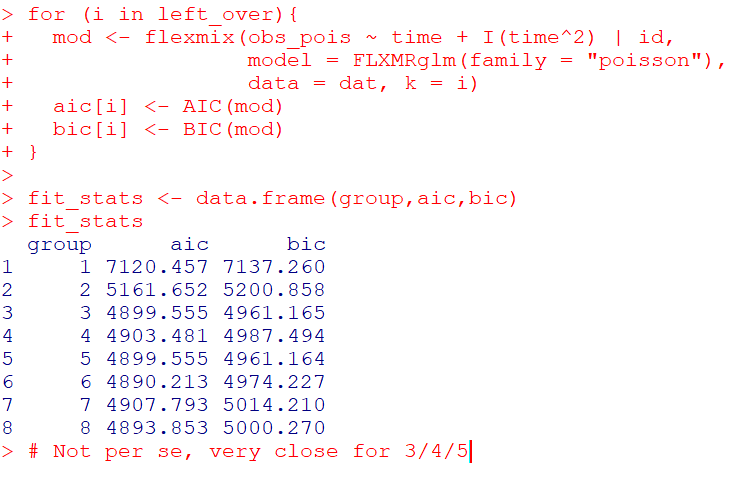
Here it actually fit the same model for 3/5 groups (sometimes even if you tell flexmix to fit 5 groups, it will only return a smaller number). You can see that the fit stats for group 4 through are almost the same. So while AIC/BIC did technically pick the right number in this simulated example, it is cutting the margin pretty close to picking 4 groups in this data instead of 3.

So the simulation Skardhamar (2010) did was slightly different than this so far. What he did was simulate data with no underlying trajectory groups, and then showed GBTM tended to spit out solutions. Here I will show that is the case as well. I simulate random intercepts and a simple linear trend over time.

################################################
# Simulate random effects model
library(lme4)
rand_eff <- rnorm(n=n,0,1.5)
dat$re <- expand.grid(t=1:t,re=rand_eff)$re
dat$re_pois <- rpois(n=n*t,lambda=exp(dat$sel_mu))
dat$mu_re <- 3 + -0.2*time + dat$re
dat$re_pois <- rpois(n=n*t,lambda=exp(dat$mu_re))

re_mod <- glmer(re_pois ~ 1 + time + (1 | id), 
                data = dat, family = poisson(link = "log"))
summary(re_mod)
################################################

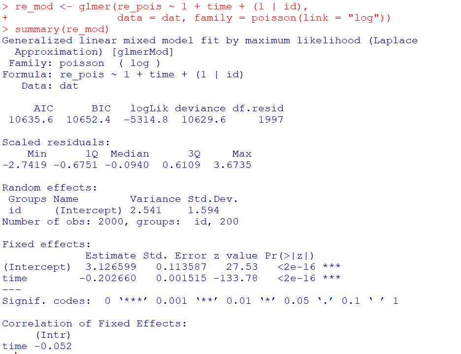
So you can see that the random effects model is all fine and dandy – recovers both the fixed coefficients, as well as estimates the correct variance for the random intercepts.

So here I go and see how the AIC/BIC compares for the random effects models vs GBTM models for 1 to 8 groups (I stuff the random effects model in the first row for group 0):

################################################
# Test AIC/BIC for random effects vs GBTM
group <- 0:8
left_over <- 1:8
aic <- rep(-1, 9)
bic <- rep(-1, 9)
aic[1] <- AIC(re_mod)
bic[1] <- BIC(re_mod)

for (i in left_over){
  mod <- flexmix(re_pois ~ time + I(time^2) | id, 
                 model = FLXMRglm(family = "poisson"),
                 data = dat, k = i)
  aic[i+1] <- AIC(mod)
  bic[i+1] <- BIC(mod)
}

fit_stats <- data.frame(group,aic,bic)
fit_stats
################################################

So it ends up flexmix will not give us any more solutions than 2 groups. But that the random effect fit is so much smaller (either by AIC/BIC) than the GBTM you wouldn’t likely make that mistake here.

I am not 100% sure how well we can rely on AIC/BIC for these different models (R does not count the individual intercepts as a degree of freedom here, so k=3 instead of k=203). But no reasonable accounting of k would flip the AIC/BIC results for these particular simulations.

One of the things I will need to experiment with more, I really like the idea of using out of sample data to validate these models instead of AIC/BIC – no different than how Nielsen et al. (2014) use leave one out CV. I am not 100% sure if that is possible in this set up with flexmix, will need to investigate more. (You can have different types of cross validation in that context, leave entire groups out, or forecast missing data within an observed group.)

References

Adepeju, M., Langton, S., & Bannister, J. (2021). Anchored k-medoids: a novel adaptation of k-medoids further refined to measure long-term instability in the exposure to crime. Journal of Computational Social Science, 1-26.

Grün, B., & Leisch, F. (2007). Fitting finite mixtures of generalized linear regressions in R. Computational Statistics & Data Analysis, 51(11), 5247-5252.

Curman, A. S., Andresen, M. A., & Brantingham, P. J. (2015). Crime and place: A longitudinal examination of street segment patterns in Vancouver, BC. Journal of Quantitative Criminology, 31(1), 127-147.

Erosheva, E. A., Matsueda, R. L., & Telesca, D. (2014). Breaking bad: Two decades of life-course data analysis in criminology, developmental psychology, and beyond. Annual Review of Statistics and Its Application, 1, 301-332.

Greenberg, D. F. (2016). Criminal careers: Discrete or continuous?. Journal of Developmental and Life-Course Criminology, 2(1), 5-44.

Nielsen, J. D., Rosenthal, J. S., Sun, Y., Day, D. M., Bevc, I., & Duchesne, T. (2014). Group-based criminal trajectory analysis using cross-validation criteria. Communications in Statistics-Theory and Methods, 43(20), 4337-4356.

Skardhamar, T. (2010). Distinguishing facts and artifacts in group-based modeling. Criminology, 48(1), 295-320.

Weisburd, D., Bushway, S., Lum, C., & Yang, S. M. (2004). Trajectories of crime at places: A longitudinal study of street segments in the city of Seattle. Criminology, 42(2), 283-322.

Wheeler, A. P., Worden, R. E., & McLean, S. J. (2016). Replicating group-based trajectory models of crime at micro-places in Albany, NY. Journal of Quantitative Criminology, 32(4), 589-612.