Motivated by a recent piece by Wood and Papachristos (2019), (WP from here on) which finds if you treat an individual at high risk for gun shot victimization, they have positive spillover effects on individuals they are connected to. This creates a tricky problem in identifying the best individuals to intervene with given finite resources. This is because you may not want to just choose the people with the highest risk – the best bang for your buck will be folks who are some function of high risk and connected to others with high risk (as well as those in areas of the network not already treated).

For a simplified example consider the network below, with individuals baseline probabilities of future risk noted in the nodes. Lets say the local treatment effect reduces the probability to 0, and the spillover effect reduces the probability by half, and you can only treat 1 node. Who do you treat?

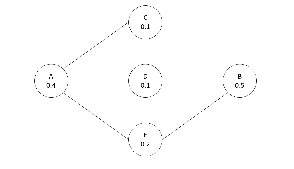
We could select the person with the highest baseline probability (B), and the reduced effect ends up being 0.5(B) + 0.1(E) = 0.6 (the 0.1 is for the spillover effect for E). We could choose node A, which is a higher baseline probability and has the most connections, and the reduced effect is 0.4(A) + 0.05(C) + 0.05(D) + 0.1(E) = 0.6. But it ends up in this network the optimal node to choose is E, because the spillovers to A and B justify choosing a lower probability individual, 0.2(E) + 0.2(A) + 0.25(B) = 0.65.

Using this idea of a local effect and a spillover effect, I formulated an integer linear program with the same idea of a local treatment effect and a spillover effect:

Where  is the reduction in the probability due to the local effect, and  is the reduction in the probability due to the spillover effect. These probabilities are fixed values you know at the onset, e.g. estimated from some model like in Wheeler, Worden, and Silver (2019) (and Papachristos has related work using the network itself to estimate risk). Each node, i, then gets two decision variables;  will equal 1 if that node is treated, and  will equal 1 if the node gets a spillover effect (depending on who is treated). Actually the findings in WP show that these effects are not additive (you don’t get extra effects if you are treated and your neighbors are treated, or if you have multiple neighbors treated), and this makes it easier to keep the problem on the probability scale. So we then have our constraints:

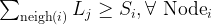
Constraint 1 is that these are binary 0/1 decision variables. Constraint 2 is we limit the number of people treated to K (a value that we choose). Constraint 3 ensures that if a local decision variable is set to 1, then the spillover variable has to be set to 0. If the local is 0, it can be either 0 or 1. Constraint 4 looks at the neighbor relations. For Node i, if any of its neighbors local treated decision variable is set to 1, the Spillover decision variable can be set to 1.

So in the end, if the number of nodes is n, we have 2*n decision variables and 2*n + 1 constraints, I find it easier just to look at code sometimes, so here is this simple network and problem formulated in python using networkx and pulp. (Here is a full file of the code and data used in this post.) (Update: I swear I’ve edited this inline code snippet multiple times, if it does not appear I have coded constraints 3 & 4, check out the above linked code file. Maybe it is causing problems being rendered.)

####################################################
import pulp
import networkx

Nodes = ['a','b','c','d','e']
Edges = [('a','c'),
         ('a','d'),
         ('a','e'),
         ('b','e')]

p_l = {'a': 0.4, 'b': 0.5, 'c': 0.1, 'd': 0.1,'e': 0.2}
p_s = {'a': 0.2, 'b': 0.25, 'c': 0.05, 'd': 0.05,'e': 0.1}
K = 1

G = networkx.Graph()
G.add_edges_from(Edges)

P = pulp.LpProblem("Choosing Network Intervention", pulp.LpMaximize)
L = pulp.LpVariable.dicts("Treated Units", [i for i in Nodes], lowBound=0, upBound=1, cat=pulp.LpInteger)
S = pulp.LpVariable.dicts("Spillover Units", [i for i in Nodes], lowBound=0, upBound=1, cat=pulp.LpInteger)

P += pulp.lpSum( p_l[i]*L[i] + p_s[i]*S[i] for i in Nodes)
P += pulp.lpSum( L[i] for i in Nodes ) == K

for i in Nodes:
    P += pulp.lpSum( S[i] ) <= 1 + -1*L[i]
    ne = G.neighbors(i)
    P += pulp.lpSum( L[j] for j in ne ) >= S[i]

P.solve()

#Should select e for local, and a & b for spillover
print(pulp.value(P.objective))
print(pulp.LpStatus[P.status])

for n in Nodes:
    print([n,L[n].varValue,S[n].varValue])
####################################################

And this returns the correct results, that node E is chosen in this example, and A and B have the spillover effects. In the linked code I provided a nicer function to just pipe in your network, your two probability reduction estimates, and the number of treated units, and it will pipe out the results for you.

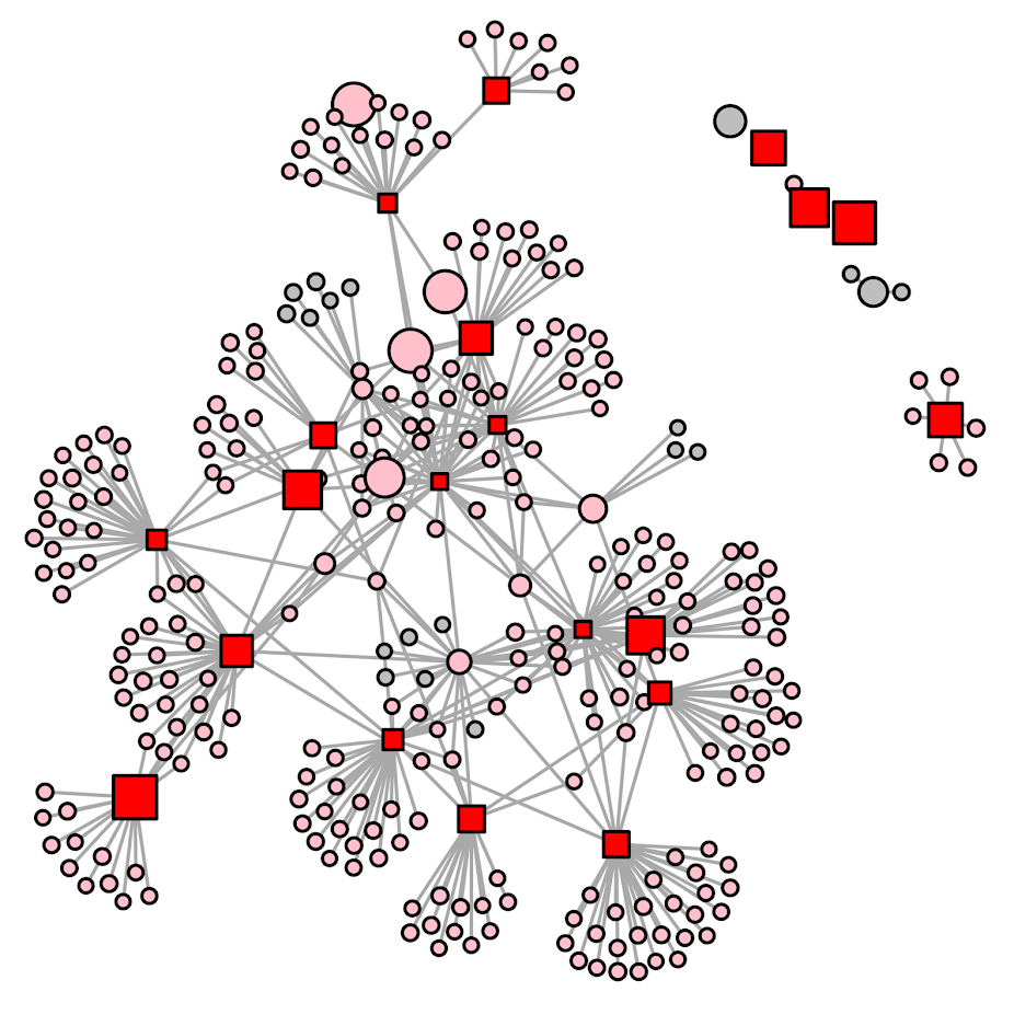
For an example with a larger network for just proof of concept, I conducted the same analysis, choosing 20 people to treat in a network of 311 nodes I pulled from Rostami and Mondani (2015). I simulated some baseline probabilities to pipe in, and made it so the local treatment effect was a 50% reduction in the probability, and a spillover effect was a 20% reduction. Here red squares are treated, pink circles are the spill-over, and non-treated are grey circles. It did not always choose the locally highest probability (largest nodes), but did tend to choose highly connected folks also with a high probability (but also chose some isolate nodes with a high probability as well).

This problem is solved in an instant. And I think out of the box this will work for even large networks of say over 100,000 nodes (I have let CPLEX churn on problems with near half a million decision variables on my desktop overnight). I need to check myself to make 100% sure though. A simple way to make the problem smaller if needed though is to conduct the analysis on subsets of connected components, and then shuffle the results back together.

Looking at the results, it is very similar to my choosing representatives work (Wheeler et al., 2019), and I think you could get similar results with just piping in 1’s for each of the local and spillover probabilities. One of the things I want to work on going forward though is treatment non-compliance. So if we are talking about giving some of these folks social services, they don’t always take up your offer (this is a problem in choose rep’s for call ins as well). WP actually relied on this to draw control nodes in their analysis. I thought for a bit the problem with treatment non-compliance in this setting was intractable, but another paper on a totally different topic (Bogle et al., 2019) has given me some recent hope that it can be solved.

This same idea is also is related to hot spots policing (think spatial diffusion of benefits). And I have some ideas about that to work on in the future as well (e.g. how wide of net to cast when doing hot spots interventions given geographical constraints).

References

• Bogle, J., Bhatia, N., Ghobadi, M., Menache, I., Bjørner, N., Valadarsky, A., & Schapira, M. (2019). TEAVAR: striking the right utilization-availability balance in WAN traffic engineering. In Proceedings of the ACM Special Interest Group on Data Communication (pp. 29-43).
• Rostami, A., & Mondani, H. (2015). The complexity of crime network data: A case study of its consequences for crime control and the study of networks. PloS ONE, 10(3), e0119309.
• Wheeler, A. P., McLean, S. J., Becker, K. J., & Worden, R. E. (2019). Choosing Representatives to Deliver the Message in a Group Violence Intervention. Justice Evaluation Journal, Online First.
• Wheeler, A. P., Worden, R. E., & Silver, J. R. (2019). The Accuracy of the Violent Offender Identification Directive Tool to Predict Future Gun Violence. Criminal Justice and Behavior, 46(5), 770-788.
• Wood, G., & Papachristos, A. V. (2019). Reducing gunshot victimization in high-risk social networks through direct and spillover effects. Nature Human Behaviour, 1-7.