Learning a fair loss function in pytorch

Most of the time when we are talking about deep learning, we are discussing really complicated architectures – essentially complicated sets of (mostly linear) equations. A second innovation in the application of deep learning though is the use of back propagation to fit under-determined systems. Basically you can feed these systems fairly complicated loss functions, and they will chug along with no problem. See a prior blog post of mine of creating simple regression weights for example.

Recently in the NIJ challenge, I used pytorch and the non-linear fairness function defined by NIJ. In the end me and Gio used an XGBoost model, because the data actually do not have very large differences in false positive rates between racial groups. I figured I would share my example here though for illustration of using pytorch to learn a complicated loss function that has fairness constraints. And here is a link to the data and code to follow along if you want.

First, in text math the NIJ fairness function was calculated as (1 - BS)*(1 - FP_diff), where BS is the Brier Score and FP_diff is the absolute difference in false positive rates between the two groups. My pytorch code to create this loss function looks like this (see the pytorch_mods.py file):

# brier score loss function with fairness constraint
def brier_fair(pred,obs,minority,thresh=0.5):
    bs = ((pred - obs)**2).mean()
    over = 1*(pred > thresh)
    majority = 1*(minority == 0)
    fp = 1*over*(obs == 0)
    min_tot = (over*minority).sum().clamp(1)
    maj_tot = (over*majority).sum().clamp(1)
    min_fp = (fp*minority).sum()
    maj_fp = (fp*majority).sum()
    min_rate = min_fp/min_tot
    maj_rate = maj_fp/maj_tot
    diff_rate = torch.abs(min_rate - maj_rate)
    fin_score = (1 - bs)*(1 - diff_rate)
    return -fin_score

I have my functions all stashed in different py files. But here is an example of loading up all my functions, and fitting my pytorch model to the training recidivism data. Here I set the threshold to 25% instead of 50% like the NIJ competition. Overall the model is very similar to a linear regression model.

import data_prep as dp
import fairness_funcs as ff
import pytorch_mods as pt

# Get the train/test data
train, test = dp.get_y1_data()
y_var = 'Recidivism_Arrest_Year1'
min_var = 'Race' # 0 is White, 1 is Black
x_vars = list(train)
x_vars.remove(y_var)

# Model learning fair loss function
m2 = pt.pytorchLogit(loss='brier_fair',activate='ident',
                     minority=min_var,threshold=0.25)
m2.fit(train[x_vars],train[y_var])

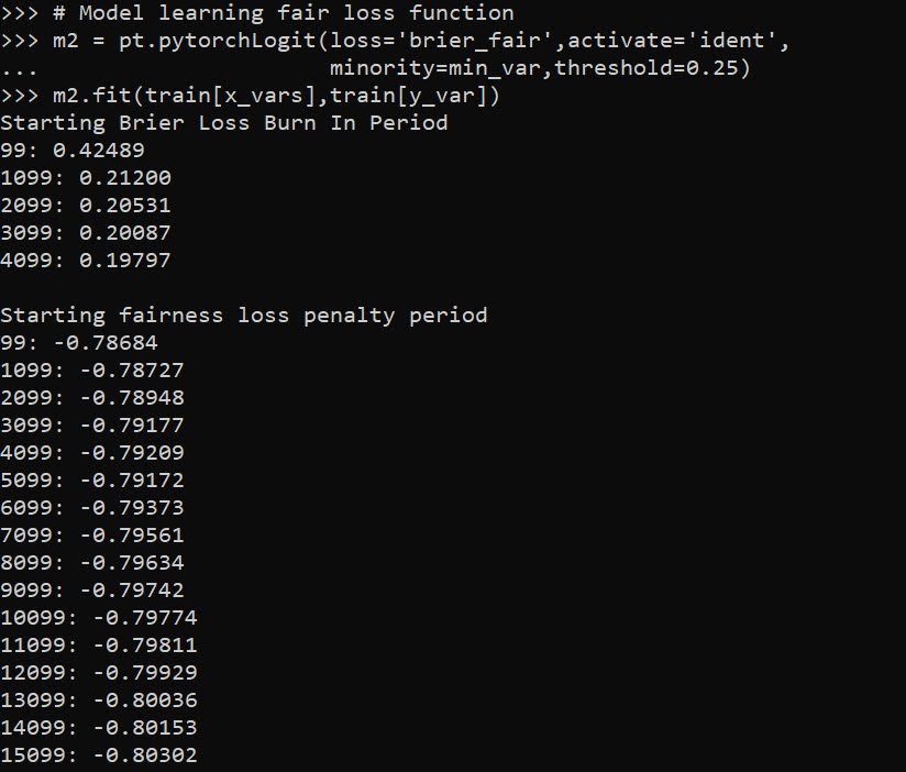
I have a burn in start to get good initial parameter estimates with a more normal loss function before going into the more complicated function. Another approach would be to initialize the weights to the solution for a linear regression equation though. After that burn in though it goes into the NIJ defined fairness loss function.

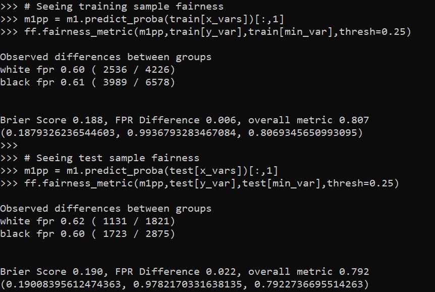
Now I have functions to see how the different model metrics in whatever sample. Here you can see the model is quite balanced in terms of false positive rates in the training sample:

# Seeing training sample fairness
m2pp = m2.predict_proba(train[x_vars])[:,1]
ff.fairness_metric(m2pp,train[y_var],train[min_var],thresh=0.25)

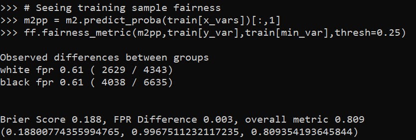
But of course in the out of sample test data it is not perfectly balanced. In general you won’t be able to ensure perfect balance in whatever fairness metrics out of sample.

# Seeing test sample fairness
m2pp = m2.predict_proba(test[x_vars])[:,1]
ff.fairness_metric(m2pp,test[y_var],test[min_var],thresh=0.25)

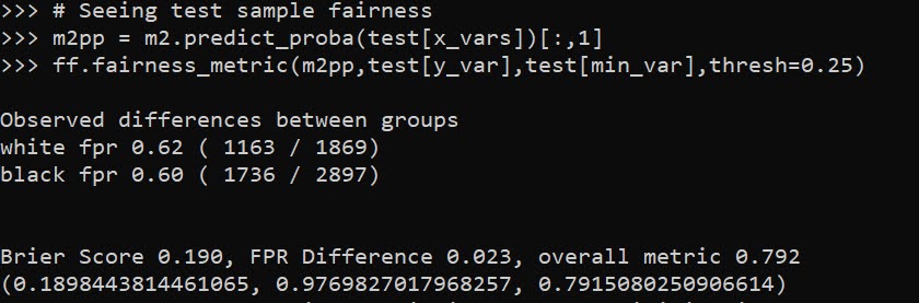
It actually ends up that the difference in false positive rates between the two racial groups, even in models that do not incorporate the fairness constraint in the loss function, are quite similar. Here is a model using the same architecture but just the usual Brier Score loss. (Code not shown, see the m1 model in the 01_AnalysisFair.py file in the shared dropbox link earlier.)

You can read mine and Gio’s paper (or George Mohler and Mike Porter’s paper) about why this particular fairness function is not the greatest. In general it probably makes more sense to use an additive fairness loss instead of multiplicative, but in this dataset it won’t matter very much no matter how you slice it in terms of false positive rates. (It appears in retrospect the Compas data that started the whole false positive thing is somewhat idiosyncratic.)

There are other potential oddities that can occur with such fair loss functions. For example if you had the choice between false positive rates for (white,black) of (0.62,0.60) vs (0.62,0.62), the latter is more fair, but the minority class is worse off. It may make more sense to have an error metric that sets the max false positive rate you want, and then just has weights for different groups to push them down to that set threshold.

These aren’t damning critiques of fair loss functions (these can be amended/changed to behave better), but in the end defining fair loss functions will be very tricky. Both for empirical reasons as well as for ethical ones – they will ultimately involve quite a few trade-offs.

genrules: using a genetic algo to find high risk cases

So I recently participated in the Decoding Maternal Morbidity Data Challenge. I did not win, but will share my work anyway. I created a genetic algorithm in python to identify sets of association rules that result in high relative risks, genrules. Here I intentionally used a genetic algorithm, with the idea I wanted not just one final model, but a host of different potential rules with the goal of exploratory data analysis.

You can go see how it works by checking out the notebook using the nuMoM2b data (which you have to request, I cannot upload that to github). Here are rules I found to predict high relative risk for infections:

And I have other code to summarize these, it happens to govt insurance is very commonly in the set of rules found.

I actually like it better just as a convenient tool (that can take weights), and go through every possible permutation of a set of categorical data. I uploaded a second notebook showing off NIBRS and predicting officer assaults (see my prior blog post on this).

So here one of the rules is stolen property, and the assailant using their motor vehicle as a weapon. So perhaps people running with stolen property in a vehicle? (While I built quite a bit of machinery to look through higher level rules, why bother with higher sets than 3 variables in the vast majority of circumstances.)

This shows the risk of competing in challenges, so a few weekends lost with no reward. This was a fuzzy competition, and something that appears I misread was in the various notes the challenge asked for the creation of novel algorithms. It appears from the titles of the winners people just used typical machine learning approaches and did a deep dive into the data. I did the opposite, created a general tool that could be used by many (who are better experts on the topical material than me).

Also note this approach is very data mining. While I use p-values as a mechanism to penalize too complicated of outcomes in the genetic algorithm, I wouldn’t take those at face value. With large datasets you will always mine some sets that are ultimately confounded.

Regression Discontinuity Designs

Regression Discontinuity Designs (RDD) are one way to evaluate predictive model systems with causal outcomes associated with what you do with that information. For a hypothetical example, imagine you have a predictive model assessing the probability that you will be diagnosed with diabetes in the next two years. Those that score above 30% probability get assigned a caseworker, to try to prevent that individual from contracting diabetes. How do you know how effective that caseworker is in reducing diabetes in those high risk individuals?

The RDD design works like this – you have your running variable (here the predicted probability), and the threshold (over 30%) that gets assigned a treatment. You estimate the probability of the actual outcome (it may be other outcomes besides just future diabetes, such as the caseworker may simply reduce overall medical costs even if the person still ends up being diagnosed with diabetes). You then estimate the dip in the predicted outcome just before and just after the threshold. The difference in those two curves is the estimated effect.

Here is an example graph illustrating (with fake data I made, see the end of the post). The bump in the line (going from the blue to the red) is then the average treatment effect of being assigned a caseworker, taking into account the underlying trend that higher risk people here are more likely to have higher medical bills.

A few things to note about RDD – so there is a tension between estimating the underlying curve and the counterfactual bump at the threshold. Theoretically values closer to the threshold should be more relevant, so some (see the Wikipedia article linked earlier) try to estimate non-linear weighted curves, giving cases closer to the threshold higher weights. This often produces strange artifacts (that Andrew Gelman likes to point out on his blog) that can miss-estimate the RDD effect. This is clearly the case in noisy data if the line dips just before the threshold and curves up right after the threshold.

So you can see in my code at the end I prefer to estimate this using splines, as opposed to weighted estimators that have a bit of noise. (Maybe someday I will code up a solution to do out of sample predictive evaluations for this as an additional check.) And with this approach it is easy to incorporate other covariates (and look at treatment heterogeneity if you want). Note that while wikipedia says the weighted estimator is non-parametric this is laughably wrong (it is two straight lines in their formulation, a quite restrictive for actually) – while I can see some theoretical justification for the weighted estimators, in practice these are quite noisy and not very robust to minor changes in the weights (and you always need to make some parametric assumptions in this design, both for the underlying curve as well as the standard error around the threshold bump).

There are additional design details you need to be worried about, such as fuzzy treatments or self selection. E.g. if a person can fudge the numbers a bit and choose which side of the line they are on, it can cause issues with this design. In those cases there may be a reasonable workaround (e.g. an instrumental variable design), but the jist of the research design will be the same.

Last but not least, to actually conduct this analysis you need to cache the original continuous prediction. In trying to find real data for this blog post, many criminal justice examples of risk assessment people only end up saving the final categories (low, medium, high) and not the original continuous risk instrument.

If folks have a good public data example that I could show with real data please let me know! Scouting for a bit (either parole/probabation risk assessment, or spatial predictive policing) has not turned up any very good examples for me to construct examples with (also health examples would be fine as well).


This is the simulated data (in python), the RDD graph, and the statsmodel code for how I estimate the RDD bump effect. You could of course do more fancy things (such as penalize the derivatives for the splines), but this I think would be a good way to estimate the RDD effect in many designs where appropriate.

from matplotlib import pyplot as plt
import numpy as np
import pandas as pd
import statsmodels.api as sm
import statsmodels.formula.api as smf

########################################
# Simulating data
np.random.seed(10)
n_cases = 3000 # total number of cases
# pretend this is predicted prob
prob = np.random.beta(3,10,size=n_cases)
# pretend this is med costs over a year
med_cost = 3000 + 5000*prob + -500*(prob > 0.3) + np.random.normal(0,500,n_cases)
df = pd.DataFrame(zip(prob,med_cost), columns=['Prob','MedCost'])
# could do something fancier with non-linear effects for prob
########################################

########################################
# Fitting regression model

# Knots are small distance from threshold
# (Could also do a knot right on threshold)
mod = smf.ols(formula='MedCost ~ bs(Prob,knots=[0.2,0.25,0.35,0.4]) + I(Prob > 0.3)', data=df)
res = mod.fit()
print(res.summary())
########################################

########################################
# Plotting fit

# Getting standard errors
prob_se = res.get_prediction().summary_frame()
prob_se['Prob'] = prob
prob_se.sort_values(by='Prob',inplace=True,ignore_index=True)
low = prob_se[prob_se['Prob'] <= 0.3].copy()
high = prob_se[prob_se['Prob'] > 0.3].copy()

# Getting effect for threshold bump
coef = res.summary2().tables[1]
ci = coef.iloc[1,4:6].astype(int).to_list()

fig, ax = plt.subplots(figsize=(6,4))
ax.scatter(df['Prob'], df['MedCost'], c='grey',
           edgecolor='k', alpha=0.15, s=5, zorder=1)
ax.axvline(0.3, linestyle='solid', alpha=1.0, 
           color='k',linewidth=1, zorder=2)
ax.fill_between(low['Prob'],low['mean_ci_lower'],
                low['mean_ci_upper'],alpha=0.6,
                zorder=3, color='darkblue')
ax.fill_between(high['Prob'],high['mean_ci_lower'],
                high['mean_ci_upper'],alpha=0.6,
                zorder=3, color='red')
ax.set_xlabel('Predicted Prob Diabetes')
ax.set_ylabel('Medical Costs')
ax.set_title(f'RDD Reduced Cost Estimate {ci[0]} to {ci[1]} (95% CI)')
ax.text(0.3,6500,'Threshold',rotation=90, size=9,
         ha="center", va="center",
         bbox=dict(boxstyle="round", ec='k',fc='grey'))
plt.savefig('RDD.png', dpi=500, bbox_inches='tight')
########################################

pre-commit hooks and github actions

In keeping up with learning about code development in python and R, two things I have added to my retenmod python package recently are pre-commit hooks and github actions. I am not going to give a code example here, you can google pre-commit python black flake and get like a dozen different blog posts to describe the process. Ditto for github actions. I think it is good to do some googling on the processes, and then you can see the final yaml files I have made to do either process:

The idea behind pre-commit, is that it runs a set of commands to check your py files before you commit your changes to github on your local system. So here the pre-commit I created for this package does three things:

  • runs black code formatter for python (formats whitespace nicely where it can)
  • runs flake8 checks (checks whether py files meet pep standards)
  • updates my readme document

Note one thing I want to be able to do but cannot currently with pre-commit is to update all jupyter notebooks in place as well. Unfortunately this does not work, as notebooks generate some time meta-data under the hood (so the file is modified, and fails the test). There is probably a way to fix this (maybe some smart config via nbdime), but it is not a big deal for me at the moment. But it works fine executing notebooks and saving to different files, so the readme hook in that example works just fine. (And won’t be as painful as say for Rmarkdown as for Jupyter with that time meta-data.)

Pre-commit hooks run on your local system, so you might not want to have it do pytests. My retenmod package though is tiny (intentionally did it as a very simple example to learn). At work I do development on both a windows machine and Red Hat virtual machines, and fortunately so far have not had issues with needing different yaml files, although I could potentially seeing that happen in more complicated set ups. Although if that were the case, I would like just not install on windows (I use local windows laptop to edit powerpoint presentations, and use Red Hat for pretty much everything else).

Github actions does not run on your personal machine, but runs after you have pushed your changes to github. And then github basically spins up virtual environments and does whatever tests. This makes sense for package development, to make sure your package can be installed on multiple operating systems. And you can run other unit tests at this stage on those systems as well. But for certain tests that only make sense on your local system (say functions to generate database connections) github actions will not make sense.

Next up I will need to learn whether it makes sense to generate artifacts via github actions (for that Jupyter notebook example where pre-commit is not working so well?). Also I have never really figured out sphinx docs for python. So I will see if I can get that up and running as well for this retenmod package.

Generating multiple solutions for linear programs

I had a question the other day on my TURF analysis about generating not just the single best solution for a linear programming problem, but multiple solutions. This is one arena I like the way people typically do genetic algorithms, in that they have a leaderboard with multiple top solutions. Which is nice for exploratory data analysis.

This example though it is pretty easy to amend the linear program to return exact solutions by generating lazy constraints. (And because the program is fast, you might as well do it this way as well to get an exact answer.) The way it works here, we have decision variables for products selected. You run the linear program, and then collect the k products selected, then add a constraint to the model in the form of:

Sum(Product_k) <= k-1 

Then rerun the model with this constraint, get the solution, and then repeat. This constraint makes it so the group of decision variables selected cannot be replicated (and in the forbidden set). Python’s pulp makes this quite easy, and here is a function to estimate the TURF model I showed in that prior blog post, but generate this multiple leaderboard:

import pandas as pd
import pulp

# Function to get solution from turf model
def get_solution(prod_dec,prod_ind):
    '''
    prod_dec - decision variables for products
    prod_ind - indices for products
    '''
    picked = []
    for j in prod_ind:
        if prod_dec[j].varValue >= 0.99:
            picked.append(j)
    return picked

# Larger function to set up turf model 
# And generate multiple solutions
def turf(data,k,solutions):
    '''
    data - dataframe with 0/1 selected items
    k - integer for products selected
    solutions - integer for number of potential solutions to return
    '''
    # Indices for Dec variables
    Cust = data.index
    Prod = list(data)
    # Problem and Decision Variables
    P = pulp.LpProblem("TURF", pulp.LpMaximize)
    Cu = pulp.LpVariable.dicts("Customers Reached", [i for i in Cust], lowBound=0, upBound=1, cat=pulp.LpInteger)
    Pr = pulp.LpVariable.dicts("Products Selected", [j for j in Prod], lowBound=0, upBound=1, cat=pulp.LpInteger)
    # Objective Function (assumes weight = 1 for all rows)
    P += pulp.lpSum(Cu[i] for i in Cust)
    # Reached Constraint
    for i in Cust:
        #Get the products selected
        p_sel = data.loc[i] == 1
        sel_prod = list(p_sel.index[p_sel])
        #Set the constraint
        P += Cu[i] <= pulp.lpSum(Pr[j] for j in sel_prod)
    # Total number of products selected constraint
    P += pulp.lpSum(Pr[j] for j in Prod) == k
    # Solve the equation multiple times, add constraints
    res = []
    km1 = k - 1
    for _ in range(solutions):
        P.solve()
        pi = get_solution(Pr,Prod)
        # Lazy constraint
        P += pulp.lpSum(Pr[j] for j in pi) <= km1
        # Add in objective
        pi.append(pulp.value(P.objective))
        res.append(pi)
    # Turn results into nice dataframe
    cols = ['Prod' + str(i+1) for i in range(k)]
    res_df = pd.DataFrame(res, columns=cols+['Reach'])
    res_df['Reach'] = res_df['Reach'].astype(int)
    return res_df

And now we can simply read in our data, turn it into binary 0/1, and then generate the multiple solutions.

#This is simulated data from XLStat
#https://help.xlstat.com/s/article/turf-analysis-in-excel-tutorial?language=en_US
prod_data = pd.read_csv('demoTURF.csv',index_col=0)

#Replacing the likert scale data with 0/1
prod_bin = 1*(prod_data > 3)

# Get Top 10 solutions
top10 = turf(data=prod_bin,k=5,solutions=10)
print(top10)

Which generates the results:

>>> print(top10)
        Prod1       Prod2       Prod3       Prod4       Prod5  Reach
0   Product 4  Product 10  Product 15  Product 21  Product 25    129
1   Product 3  Product 15  Product 16  Product 25  Product 26    129
2   Product 4  Product 14  Product 15  Product 16  Product 26    129
3  Product 14  Product 15  Product 16  Product 23  Product 26    129
4   Product 3  Product 15  Product 21  Product 25  Product 26    129
5  Product 10  Product 15  Product 21  Product 23  Product 25    129
6   Product 4  Product 10  Product 15  Product 16  Product 27    129
7  Product 10  Product 15  Product 16  Product 23  Product 27    129
8   Product 3  Product 10  Product 15  Product 21  Product 25    128
9   Product 4  Product 10  Product 15  Product 21  Product 27    128

I haven’t checked too closely, but this looks to me offhand like the same top 8 solutions (with a reach of 129) as the XLStat website. The last two rows are different, likely because there are further ties.

For TURF analysis, you may actually consider a lazy constraint in the form of:

Product_k = 0 for each k

This is more restrictive, but if you have a very large pool of products, will ensure that each set of products selected are entirely different (so a unique set of 5 products for every row). Or you may consider a constraint in terms of customers reached instead of on products, so if solution 1 reaches 129, you filter those rows out and only count newly reached people in subsequent solutions. This ensures each row of the leaderboard above reaches different people than the prior rows.

Extending sklearns OrdinalEncoder

I’ve used a variant of this for a few different projects, so figured it was worth sharing. Sklearn’s OrdinalEncoder is close, but not quite what I want for a few different scenarios. Those are:

  • mixed input data types
  • missing data support (which can vary across the mixed input types)
  • the ability to limit encoding of rare categories (useful for regression models)

So I have scripted up a simple new class, what I call SimpleOrdEnc(), and can share it here in the blog post.

from sklearn.preprocessing import OrdinalEncoder
import numpy as np
import pandas as pd

class SimpleOrdEnc():
    def __init__(self, dtype=int, unknown_value=-1, lim_k=None,
                 lim_count=None):
        self.unknown_value = unknown_value
        self.dtype = dtype
        self.lim_k = lim_k
        self.lim_count = lim_count
        self.vars = None
        self.soe = None
    def fit(self, X):
        self.vars = list(X)
        # Now creating fit for each variable
        res_oe = {}
        for v in list(X):
            res_oe[v] = OrdinalEncoder(dtype=self.dtype,
                handle_unknown='use_encoded_value',
                        unknown_value=self.unknown_value)
            # Get unique values minus missing
            xc = X[v].value_counts().reset_index()
            # If lim_k, only taking top K value
            if self.lim_k:
                top_k = self.lim_k - 1
                un_vals = xc.loc[0:top_k,:]
            # If count, using that to filter
            elif self.lim_count:
                un_vals = xc[xc[v] >= self.lim_count].copy()
            # If neither
            else:
                un_vals = xc
            # Now fitting the encoder for one variable
            res_oe[v].fit( un_vals[['index']] )
        # Appending back to the big class
        self.soe = res_oe
    # Defining transform/inverse_transform classes
    def transform(self, X):
        xcop = X[self.vars].copy()
        for v in self.vars:
            xcop[v] = self.soe[v].transform( X[[v]].fillna(self.unknown_value) )
        return xcop
    def inverse_transform(self, X):
        xcop = X[self.vars].copy()
        for v in self.vars:
            xcop[v] = self.soe[v].inverse_transform( X[[v]].fillna(self.unknown_value) )
        return xcop

This works mostly the same way that other sklearn objects do. You instantiate the object, then call fit, transform, inverse_transform, etc. Under the hood it just turns the data into a collection of ordinal encoders, but does a few things. One is that it strips missing values from the original fit data – so out of the box you do not need to do anything like x.fillna(-1), it just works. It is on you though to choose a missing unknown value that does not collide with potential encoded or decoded values. (Also for fit it should be a pandas dataframe, weird stuff will happen if you pass other numpy objects or lists.)

The second are the lim_k or the lim_count arguments. This is useful if you want to encode rare categories as another value. lim_k is if you want to say keep the top 20 categories in the fitted dataset. lim_count sets the threshold at how many cases are in the data, e.g. if you have at least 100 keep it. lim_k takes precedence over lim_count, so if you specify both lim_count is ignored.

These args also confound the missing values, so missing (even if it is common in the data), gets assiged to the ‘other’ category in this encoding. If that is not the behavior you want, I don’t see any way around not explicitly using fillna() before all this.

So here is a simple example use case:

x1 = [1,2,3]
x2 = ['a','b','c']
x3 = ['z','z',None]
x4 = [4,np.nan,5]

x = pd.DataFrame(zip(x1,x2,x3,x4),columns=['x1','x2','x3','x4'])
print(x)

oe = SimpleOrdEnc()
oe.fit(x)

# Transform to the same data
tx = oe.transform(x)
print(tx)

# Inverse transform gives you None
ix = oe.inverse_transform(tx)
print(ix)

So you can see this handles missing input data, but the inverse transform always returns None values for missing. The fit method though returns numeric encoded columns with the same variable names. I default to missing values of -1 as light boost (and I think catboost as well), have those as the default missing data values for categorical data.

Here is an example limiting the output to only categories that have at least 10 observations, and setting the missing data value to 99 instead of -1.

size = 1000
x1 = np.random.choice(['a','b','c'], size).tolist()
x2 = np.random.choice([1, np.nan, 2], size, p=[0.8,0.18,0.02]).tolist()
x3 = np.random.choice(['z','y','x','w',np.nan], size, p=[0.8,0.15,0.04, 0.005, 0.005]).tolist()
x = pd.DataFrame(zip(x1,x2,x3),columns=['x1','x2','x3'])

oe = SimpleOrdEnc(lim_count=10, unknown_value=99)
oe.fit(x)

# Checking with a simpler data frame

x1 = ['a','b','c','d',None,]
x2 = [1,2,-1,4,np.nan]
x3 = ['z','y','x','w','v']
sx = pd.DataFrame(zip(x1,x2,x3),columns=['x1','x2','x3'])

oe.transform(sx)

Because the class is all wrapped up in one object, you can then use pickle to save the object/use later in pipelines. If I know I want to test out specific regression models with my data, I often use the lim_count to make sure I am not keeping a bunch of small dangles of high cardinality data. (Often in my data I use missing data is rare enough I don’t even want to worry about imputing, I rather just treat it as a rare category.)

One use case this does not work out so well though for is ICD codes in wide format. Will need to write another blog post about that. But often will just reshape wide to long to fit these encoders.

Using Jupyter Notebooks to make nice README’s for GitHub

Working on my R package ptools, the devtools folks have you make a readme R markdown file to compile to a nice readme markdown file for github. I thought to myself that you could functionally do the same thing with juypter notebooks for python. So here is a quick example of that for my retenmod python package.

So first, here is the old readme in its entirety, rendered on Github:

You can see I have an example code snippet, but it does not actually output the results. Here is the update, where I use jupyter to render the markdown nicely:

So we have nice syntax highlighting even. (Note that the pip install code is not run in a %sh cell, it is just code formatting inside of a markdown cell.) I do like the way R markdown renders the output a bit nicer than here (I also haven’t tried with pretty pandas tables). But you can also include matplotlib images as well:

You might typically want to add in README.ipynb to your gitignore file, but here I included it in the github package so you can see what this notebook looks like. To compile the notebook to markdown is quite simple:

jupyter nbconvert --execute --to markdown README.ipynb

If you have matplotlib images, it saves them in a folder named README_files (not sure if there is a flag to change this option). To get the images to render you then also need to push that image folder into Github.

Reversion in the tech stack and why DS models fail

Hackernews recently shared a story about not using an IDE, and I feel mostly the same way. Hence the title in the post – so my current workflow for when I steal some time to work on my R package ptools my workflow looks like this, using Rterm from the shell:

I don’t have anything against RStudio, I just only have so much room in my brain. Sometimes conversations at work are like a foreign language, “How are we going to test the NiFi script from Hadoop to our Kubernetes environment” or “I can pull the docker image from JFrog, but I run out of room when extracting the image on our sandbox machine. But df says we have plenty of room on all the partitions?”.

If you notice at the top the (base) in front of the shell, that is because this is within the anaconda shell as well. So if you look at many of my past blog posts (see here for one example), I am just using the snipping tool in windows to take screenshots of the shell output in interactive mode.

I am typically just writing the code in Notepad++ (as well as this blog post) – and it is quite simple to switch between interactive copy this function/code and compiling entire scripts. Here is a screenshot of R unit tests for example.

So Notepad++ has some text highlight (for both R and python), and that is nice, but honestly not that necessary. Main thing I use is the selection of brackets to make sure they are balanced. I am sure I am missing out on some nice autocomplete features that would make me more productive, and function hints in Spyder are nice for pandas functions (I mostly use google still though for that when I need it).

I do use VS Code for development work on our headerless virtual machines at work. But that is more to replicate essentially the workflow on Windows with file explorer + Notepad++ + Shell (I am not a vim ninja – what is it esc + wq:, need to look that up everytime). I fucked up one of my git repos the other day using VS Code stuff tools, and I am just using git directly anymore. (Again this means I am the problem, not VS Code!)

Why data science projects fail?

Some more random musings, but the more I get involved and see what projects work and what don’t at work, pretty much all of the failures I have come across are due to what I will call “not modeling the right thing”. That potentially covers a bit, but quite a few are simply not understanding counterfactual reasoning and selection bias.

The modeling part (in terms of actually fitting models) is typically quite easy – you do some simple but slightly theoretically informed feature engineering and feed that info into a machine learning model that is very flexible. But maybe that is the problem, people can easily fool themselves into thinking a model looks good, but because they are modeling the wrong thing it does not result in better decision making.

Even in most of the failures I have seen, selection bias is surmountable (often just requires multiple models or models on different samples of data – reduced form for the win!). So learning how to train/test split the data, and feed your data into XGboost only takes a few classes to learn. How to know the right thing to model though takes a bit more thought.

A secondary part of the failure is not learning how to translate the model outputs into actionable decisions. But the not modeling the right thing is at the start, so makes any downstream decision not work out how you want.

Chunking it up in pandas

In the python pandas library, you can read a table (or a query) from a SQL database like this:

data = pandas.read_sql_table('tablename',db_connection)

Pandas also has an inbuilt function to return an iterator of chunks of the dataset, instead of the whole dataframe.

data_chunks = pandas.read_sql_table('tablename',db_connection,chunksize=2000)

I thought for awhile this was somewhat worthless, as I thought it still read the whole thing into memory. I have been using it though to pull new records, generate predictions, and then feed the predictions back into another table though (easier to write back to a new DB in smaller chunks).

But I actually did some tests recently and I was wrong. When using chunksize, it does not read the whole table into memory, so works like you would want. In particular, I was testing out sqlalchemy and execution_options=dict(stream_results=True) when creating the engine. Which works great for postgres – it is not needed though for every other DB I have tried so far (I will show postgres and sqlite here, at work have also tested teradata and sql server).

Here I use the python library memory_profiler and show the difference in memory usage for a database of crime incidents from Dallas PD. First in my script I load in the libraries I will be using, and then created my different engine connection strings

''' 
Tests for memory and chunking
up dataframes
'''
import sqlalchemy
import pandas as pd
from datetime import datetime
from memory_profiler import profile

# Check out https://github.com/apwheele/Blog_Code/tree/master/Python/jupyter_reports
# For where this data came from
# sqlalchemy string for SQLlite
sqli = r'sqlite:///D:\Dropbox\Dropbox\PublicCode_Git\Blog_Code\Python\jupyter_reports\DPD.sqlite'
lite_eng = sqlalchemy.create_engine(sqli)

# sqlalchemy string for postgres
pg = f'postgresql://id:pwd@localhost/dbname' #need to fill these in with your own info
pg_eng = sqlalchemy.create_engine(pg)
pg_eng_str = sqlalchemy.create_engine(pg, execution_options=dict(stream_results=True))

Next, we can make a function to either read a table all at once, or to return an iterator that chunks the data up into a tinier number of rows. We also decorate this function with the profile function to get some nice statistics later. Here I just do some random stats and accumulate them in each iteration.

@profile
def read_table(sql_con, chnk=None):
    begin_time = datetime.now()
    inc = pd.read_sql_table('incidents',sql_con,chunksize=chnk)
    # If chunk, do the calcs in iterations
    if chnk:
        tot_inc, tot_arr = 0,0
        for c in inc:
            tot_inc += c.shape[0]
            tot_arr += (c['Offense_Status'] == 'Clear by Arrest').sum()
    else:
        tot_inc = inc.shape[0]
        tot_arr = (inc['Offense_Status'] == 'Clear by Arrest').sum()
    print(f'\nsql: {sql_con}\nTotal incidents {tot_inc}\nTotal arrests {tot_arr}\nRuntime {begin_time} -- {datetime.now()}\n')

Most of the time I am using something like this for predictions or generating follow up metrics to see how well my model is doing (and rewriting those intermediate results to a table). So inside the iteration loop looks something like pred_val = predict_function(c) and pred_val.to_sql('new_table',sql_con,if_exists='append').

Now just to finish off the script, you can do run the tests if called directly:

if __name__ == "__main__":
    read_table(sqli,None)       #sqlite big table all at once
    read_table(sqli,2000)       #sqlite in chunks
    read_table(pg_eng,None)     #pg big table
    read_table(pg_eng,2000)     #pg in chunks
    read_table(pg_eng_str,2000) #pg stream in chunks

Now when running this script, you would run it as python -m memory_profiler chunk_tests.py > test_results.txt, and this will give you a nice set of print outs for each function call. So lets start with sqlite reading the entire database into memory:

sql: sqlite:///D:\Dropbox\Dropbox\PublicCode_Git\Blog_Code\Python\jupyter_reports\DPD.sqlite
Total incidents 785064
Total arrests 89741
Runtime 2021-08-11 19:22:41.652316 -- 2021-08-11 19:23:53.743702

Filename: chunk_tests.py

Line #    Mem usage    Increment  Occurences   Line Contents
============================================================
    28     82.4 MiB     82.4 MiB           1   @profile
    29                                         def read_table(sql_con, chnk=None):
    30     82.4 MiB      0.0 MiB           1       begin_time = datetime.now()
    31   4260.7 MiB   4178.3 MiB           1       inc = pd.read_sql_table('incidents',sql_con,chunksize=chnk)
    32                                             # If chunk, do the calcs in iterations
    33   4260.7 MiB      0.0 MiB           1       if chnk:
    34                                                 tot_inc, tot_arr = 0,0
    35                                                 for c in inc:
    36                                                     tot_inc += c.shape[0]
    37                                                     tot_arr += (c['Offense_Status'] == 'Clear by Arrest').sum()
    38                                             else:
    39   4260.7 MiB      0.0 MiB           1           tot_inc = inc.shape[0]
    40   4261.5 MiB      0.8 MiB           1           tot_arr = (inc['Offense_Status'] == 'Clear by Arrest').sum()
    41   4261.5 MiB      0.0 MiB           1       print(f'\nsql: {sql_con}\nTotal incidents {tot_inc}\nTotal arrests {tot_arr}\nRuntime {begin_time} -- {datetime.now()}\n')

You can see that the incident database is 785k rows (it is 100 columns as well). It takes only alittle over a minute to read in the table, but it takes up over 4 gigabytes of memory. So I can fit this in memory on my machine, but if I say added a free text comments field I might not be able to fit this in memory on my personal machine.

Now lets see what these results look like when I chunk the data up into smaller sets of only 2000 rows at a time:

sql: sqlite:///D:\Dropbox\Dropbox\PublicCode_Git\Blog_Code\Python\jupyter_reports\DPD.sqlite
Total incidents 785064
Total arrests 89741
Runtime 2021-08-11 19:23:56.475680 -- 2021-08-11 19:25:33.896884

Filename: chunk_tests.py

Line #    Mem usage    Increment  Occurences   Line Contents
============================================================
    28     91.6 MiB     91.6 MiB           1   @profile
    29                                         def read_table(sql_con, chnk=None):
    30     91.6 MiB      0.0 MiB           1       begin_time = datetime.now()
    31     91.9 MiB      0.3 MiB           1       inc = pd.read_sql_table('incidents',sql_con,chunksize=chnk)
    32                                             # If chunk, do the calcs in iterations
    33     91.9 MiB      0.0 MiB           1       if chnk:
    34     91.9 MiB      0.0 MiB           1           tot_inc, tot_arr = 0,0
    35    117.3 MiB    -69.6 MiB         394           for c in inc:
    36    117.3 MiB    -89.6 MiB         393               tot_inc += c.shape[0]
    37    117.3 MiB    -89.6 MiB         393               tot_arr += (c['Offense_Status'] == 'Clear by Arrest').sum()
    38                                             else:
    39                                                 tot_inc = inc.shape[0]
    40                                                 tot_arr = (inc['Offense_Status'] == 'Clear by Arrest').sum()
    41    112.0 MiB     -5.3 MiB           1       print(f'\nsql: {sql_con}\nTotal incidents {tot_inc}\nTotal arrests {tot_arr}\nRuntime {begin_time} -- {datetime.now()}\n')

We only end up maxing out the memory at under 120 megabytes. You can see the total function also only takes around 1.5 minutes. So it is only ~30 seconds longer to run this result in chunks than doing it all at once.

Now onto postgres, I will forego showing the results when reading in the whole table at once – it is pretty much the same as sqlite when reading the whole table at once. But here are the results for the chunks with the usual sqlalchemy connection string:

sql: Engine(postgresql://postgres:***@localhost/postgres)
Total incidents 785064
Total arrests 89741
Runtime 2021-08-11 19:26:28.454807 -- 2021-08-11 19:27:41.917612

Filename: chunk_tests.py

Line #    Mem usage    Increment  Occurences   Line Contents
============================================================
    28     51.3 MiB     51.3 MiB           1   @profile
    29                                         def read_table(sql_con, chnk=None):
    30     51.3 MiB      0.0 MiB           1       begin_time = datetime.now()
    31   2017.2 MiB   1966.0 MiB           1       inc = pd.read_sql_table('incidents',sql_con,chunksize=chnk)
    32                                             # If chunk, do the calcs in iterations
    33   2017.2 MiB      0.0 MiB           1       if chnk:
    34   2017.2 MiB      0.0 MiB           1           tot_inc, tot_arr = 0,0
    35   2056.8 MiB  -1927.3 MiB         394           for c in inc:
    36   2056.8 MiB      0.0 MiB         393               tot_inc += c.shape[0]
    37   2056.8 MiB      0.0 MiB         393               tot_arr += (c['Offense_Status'] == 'Clear by Arrest').sum()
    38                                             else:
    39                                                 tot_inc = inc.shape[0]
    40                                                 tot_arr = (inc['Offense_Status'] == 'Clear by Arrest').sum()
    41     89.9 MiB  -1966.9 MiB           1       print(f'\nsql: {sql_con}\nTotal incidents {tot_inc}\nTotal arrests {tot_arr}\nRuntime {begin_time} -- {datetime.now()}\n')

So here we get some savings, but not nearly as good as sqlite – it ends up reading in around 2 gig for the iterator. But no fear, there is a specific option when setting up the sqlalchemy string for postgres. If you pay close attention to above where I build the connection strings, the engine for this trial is pg_eng_str = sqlalchemy.create_engine(pg, execution_options=dict(stream_results=True)). And when I use the streaming results engine, here is the memory profile I get:

sql: Engine(postgresql://postgres:***@localhost/postgres)
Total incidents 785064
Total arrests 89741
Runtime 2021-08-11 19:27:41.922613 -- 2021-08-11 19:28:54.435834

Filename: chunk_tests.py

Line #    Mem usage    Increment  Occurences   Line Contents
============================================================
    28     88.8 MiB     88.8 MiB           1   @profile
    29                                         def read_table(sql_con, chnk=None):
    30     88.8 MiB      0.0 MiB           1       begin_time = datetime.now()
    31     89.6 MiB      0.8 MiB           1       inc = pd.read_sql_table('incidents',sql_con,chunksize=chnk)
    32                                             # If chunk, do the calcs in iterations
    33     89.6 MiB      0.0 MiB           1       if chnk:
    34     89.6 MiB      0.0 MiB           1           tot_inc, tot_arr = 0,0
    35    100.5 MiB   -322.6 MiB         394           for c in inc:
    36    100.5 MiB   -325.4 MiB         393               tot_inc += c.shape[0]
    37    100.5 MiB   -325.4 MiB         393               tot_arr += (c['Offense_Status'] == 'Clear by Arrest').sum()
    38                                             else:
    39                                                 tot_inc = inc.shape[0]
    40                                                 tot_arr = (inc['Offense_Status'] == 'Clear by Arrest').sum()
    41     92.3 MiB     -8.2 MiB           1       print(f'\nsql: {sql_con}\nTotal incidents {tot_inc}\nTotal arrests {tot_arr}\nRuntime {begin_time} -- {datetime.now()}\n')

Which is very similar to sqlite results.

Some workflows unfortunately are not so reducable into tiny chunks like this. E.g. say you were doing multiple time series for different groups, you would likely need to use substitution into the SQL to get one group at a time. I have done this to grab chunks of claims data one month at a time, but in many of my workflows I could just replace that with chunksize and do one read.

Some folks reading this may be thinking “this is a great use case for hadoop”. For the most part I am personally not working with that big of data, just mildly annoying at the edge of fitting into memory data. So this just do stuff in chunks works great for most of my workflows, and I don’t have to deal with the hassles of hadoop/spark.

Solving the P-Median model

Wendy Jang, my former student at UTD and now Data Scientist for the Stanislaus County Sheriff’s Dept. writes in:

Hello Andy,

I have some questions about your posting in GitHub. Honestly, I am not good at Python at all. I was playing with your python code and trying to understand the work flow. Then, I can pretty much mimic what you did; however, I encountered some errors along the way.

I was able to follow through lines but then I am stuck on PMed function. Do you know what possibly caused this error? See the screenshot below. Please advise. Thanks!

Specifically, Wendy is asking about my patrol redistricting example with workload inequality constraints. Wendy’s problem here is specifically she likely does not have CPLEX installed. CPLEX is free for academics, but unfortunately costs a bit of money for anyone else (not sure if they have cheaper licensing for public sector, looks like currently about $200 a month).

This was a good opportunity to update some of my code, so now see the two .py files in the DataCreated folder, in particular 01_pmed_class.py has a nice class function. I have additionally added in functionality to create a map, and more importantly eliminate subtours (my solution can potentially return disconnected areas). I have also added the ability to use different solvers.

For this problem CPLEX just works much better (takes around 10 minutes), but I was able to get the SCIP solver to return the same solution in around 5 hours. GLPK did not return a solution even letting it churn out for over 12 hours. I tested CBC for shorter time periods, but that appears to be a no-go as well.

So just a brief overview, the libraries I will be using (check out the end of the post for setting up the conda environment):

import pickle
import pulp
import networkx
import pandas as pd
from datetime import datetime
import matplotlib.pyplot as plt
import geopandas as gpd

class pmed():
    """
    Ar - list of areas in model
    Di - distance dictionary organized Di[a1][a2] gives the distance between areas a1 and a2
    Co - contiguity dictionary organized Co[a1] gives all the contiguous neighbors of a1 in a list
    Ca - dictionary of total number of calls, Ca[a1] gives calls in area a1
    Ta - integer number of areas to create
    In - float inequality constraint
    Th - float distance threshold to make a decision variables
    """
    def __init__(self,Ar,Di,Co,Ca,Ta,In,Th):

I do not copy-paste the entire pmed class in the blog post. It is long, but is the rewrite of my model from the paper. Next, to load in the objects I need to fit the model (which were created/pickled in the 00_PrepareData.py file).

# Loading in data
data_loc = r'D:\Dropbox\Dropbox\PublicCode_Git\PatrolRedistrict\PatrolRedistrict\DataCreated\fin_obj.pkl'
areas, dist_dict, cont_dict, call_dict, nid_invmap, MergeData = pickle.load(open(data_loc,"rb"))

# shapefile for reporting areas
carr_report = gpd.read_file(r'D:\Dropbox\Dropbox\PublicCode_Git\PatrolRedistrict\PatrolRedistrict\DataOrig\ReportingAreas.shp')

And now we can create a pmed object, which has all the info necessary, and gives us a print out of the total number of decision variables and constraints.

# Creating pmed object
pmed12 = pmed(Ar=areas,Di=dist_dict,Co=cont_dict,Ca=call_dict,Ta=12,In=0.1,Th=10)

Writing the class this way allows the user to input their own solver, and you can see it prints out the available solvers on your current machine. So to pass in the SCIOPT solver you could do pmed12.solve(solver=pulp.SCIP_CMD()), which again for this problem does find the solution, but takes 5 hours. So here I still stick with CPLEX to just illustrate the new classes functionality:

pmed12.solve(solver=pulp.CPLEX(timeLimit=30*60,msg=True))     # takes around 10 minutes

This prints out a ton of information at the command line that you do not get if you run from within Jupyter notebooks. So for debugging that is much more useful. timeLimit is in seconds, but does not include the presolve phase I believe, so some of these solvers can just get stuck on the presolve forever.

We can look at the results in a nice map if you do have geopandas installed and pass it a geopandas data frame and the key to match it on:

pmed12.map_plot(carr_report, 'PDGrid')

This map shows the new areas and different colors with a thick border, and the source area as a dot with a white outline. So here you can see that we end up having one disconnected area – a subtour in optimization parlance. I have added some methods to deal with this though:

stres = pmed12.collect_subtours()

And you can see that for one of our areas it identified a subtour. I haven’t written this to automatically resolve for subtours due to the potential length of the solving time. So here we can see the subtours have 0 calls in them. You can assign those areas to wherever and it does not change the objective function. So that is what I did in the paper and showed how in the Jupyter notebook at the main page for the github project.

So if you are using a function that takes 5 hours, I would suggest you manually fix these subtours if there is an obvious to the human eye easy solution. But here with the shorter solve time with CPLEX I can rerun the algorithm with a warm start, and it runs even faster (under 5 minutes). The .collect_subtours() method adds subtour constraints into the pulp model, so you just need to redo the solve() method to eliminate that particular subtour (I do not know if this is guaranteed to converge though for all problems).

So here in this data eliminating that one subtour results in a solution with no subtours:

pmed12.solve(solver=pulp.CPLEX_CMD(msg=False,warmStart=True))
stres = pmed12.collect_subtours()

And we can replot the result, which shows it chooses the areas that you would have assigned by eye anyway:

pmed12.map_plot(carr_report, 'PDGrid')

So again for this problem if you have CPLEX I would recommend it (have not tried Gurobi). But at least for this particular dataset SCIOPT was able to solve the problem in 5 hours. So if you are a crime analyst or someone else without academic access to CPLEX you can install the sciopt solver and give that a go for your actual data.

Note that this is based off of results for 325 subareas. So if you have more subareas it will take a longer (and if you have fewer it may be quite a bit shorter).

Setting up the Conda environment

So once you have python installed, you can typically do something like:

pip install pulp

Or via conda:

conda install pyscipopt

I often have trouble though, especially when working with the python geospatial libraries, to install geopandas, fiona, etc. So here what I do is create a new conda environment:

conda create -n linprog
conda activate linprog
conda install -c conda-forge python=3 pip pandas numpy networkx scikit-learn dbfread geopandas glpk pyscipopt pulp

And then you can run the pmedian code above in this environment. I suppose I should turn this into a python package, and I see a bunch of folks anymore are doing docker images as well with their packages in complicated environments. This is actually not that bad, minus geopandas makes things a bit tricky.