Estimating Criminal Lifetime Value

At work I am currently working on estimating/forecasting healthcare spending. Similar to work I have done on forecasting person level crime risks (Wheeler et al., 2019), I build the predictive model dataset like this:

CrimeYear2020 PriorCrimeA PriorCrimeB
     0              2          3
     1              5          0
     0              0          0

etc. So I flatten people to a single row, and as covariates include prior cumulative crime histories. Most people do this similarly in the healthcare setting, so it looks like:

SpendingYear2020 PriorComorbidA PriorComorbidB
     3000              1          2
      500              3          0
    10000              0          0

Or sometimes people do a longitudinal dataset, where it is a spending*year*person panel (see Lauffenburger et al., 2020 for an example). I find this approach annoying for a few reasons though. One, it requires arbitrary temporal binning, which is somewhat problematic in these transaction level databases. We are talking for chronic offenders a few crimes per year is quite high, and ditto in the healthcare setting a few procedures a year can be very costly. So there is not much data to estimate the underlying function over time.

A second aspect I think is bad is that it doesn’t take into account the recency of the patterns. So the variables on the right hand side can be very old or very new. And with transaction level databases it is somewhat difficult to define how to estimate the lookback – do you consider it normalized by time? The VOID paper I mentioned we evaluated the long term scores, but the PD that does that chronic offender system has two scores – one a cumulative history and another a 90 day history to attempt to deal with that issue (again ad-hoc).

One approach to this issue from marketing research I have seen from very similar types of transactions databases are models to estimate Customer Lifetime Value (Fader et al. 2005). These models in the end generate a dataset that looks like this:

Person    RecentMonths  TotalEvents AveragePurchase
  A            3             5            $50
  B            1             2           $100
  C            9             8            $25

TotalEvents should be straightforward, RecentMonths just is a measure of the time since the last purchase, and then you have the average value of the purchases. And using just this data, estimates the probability of any future purchases, as well as projects the total value of the future average purchases. So here I use an example of this approach, using the Wolfgang Philly cohort public data. I am not going into the model more specifically (read some of the Bruce Hardie notes to get a flavor).

I have created some python code to follow along and apply these same customer lifetime value estimates to chronic offender data. Most examples of weighting crime harm apply it to spatial areas (Mitchell, 2019; Wheeler & Reuter, 2021), but you can apply it the same to chronic offender lists (Liggins et al., 2019).

Example Criminal Lifetime Value in Python

First, install the lifetimes python library – Cam’s documentation is excellent and makes the data manipulation/modelling quite simple.

Here I load in the transaction level crime data, e.g. it just have person A, 1/5/1960, 1000, where the 1000 is a crime seriousness index created by Wolfgang. Then the lifetimes package has some simple functions to turn our data into the frequency/recency format.

Note that for these models, you drop the first event in the series. To build a model to do train/test, I also split the data into evens before 1962, and use 1962 as the holdout test period.

import lifetimes as lt
import pandas as pd

# Just the columns from dataset II
# ID, SeriousScore, Date
df = pd.read_csv('PhilData.csv')
df['Date'] = pd.to_datetime(df['Date'])

# Creating the cumulative data
# Having holdout for one year in future
sd = lt.utils.calibration_and_holdout_data(df,'ID','Date',
              calibration_period_end='12-31-1961',
              observation_period_end='12-31-1962',
              freq='M',
              monetary_value_col='SeriousScore')

# Only keeping people with 2+ events in prior period
sd = sd[sd['frequency_cal'] > 0].copy()
sd.head()

Recency_cal is how many months since a prior crime (starting in 1/1/1962), frequency is the total number of events (minus 1, so number of repeat events technically), and the monetary_value_cal here is the average of the crime seriousness across all the events. The way this function works, the variables with the subscript _cal are in the training period, and _holdout are events in the 1962 period. For subsequent models I subset out people with at least 2 events total in the modeling.

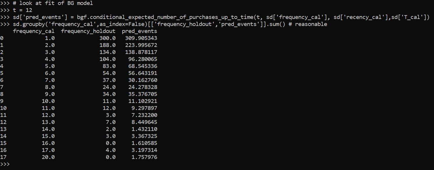
Now we can fit a model to estimate the predicted number of future crimes a person will commit – so this does not take into account the seriousness of those crimes. The final groupby statement shows the predicted number of crimes vs those actually committed, broken down by number of crimes in the training time period. You can see the model is quite well calibrated over the entire sample.

# fit BG model
bgf = lt.BetaGeoFitter(penalizer_coef=0)
bgf.fit(sd['frequency_cal'],sd['recency_cal'],sd['T_cal'])

# look at fit of BG model
t = 12
sd['pred_events'] = bgf.conditional_expected_number_of_purchases_up_to_time(t, sd['frequency_cal'], sd['recency_cal'],sd['T_cal'])
sd.groupby('frequency_cal',as_index=False)[['frequency_holdout','pred_events']].sum() # reasonable

Now we can fit a model to estimate the average crime severity score for an individual as well. Then you can project a future cumulative score for an offender (here over a horizon of 1 year), by multiple the predicted number of events times the estimate of the average severity of the events, what I label as pv here:

# See conditional seriousness
sd['pred_ser'] = ggf.conditional_expected_average_profit(
                              sd['frequency_cal'],
                              sd['monetary_value_cal'])

sd['pv'] = sd['pred_ser']*sd['pred_events']
sd['cal_tot_val'] = sd['monetary_value_holdout']*sd['frequency_holdout']
# Not great correlation, around 0.2
vc = ['frequency_holdout','monetary_value_holdout','cal_tot_val','pred_events','pv']
sd[vc].corr()

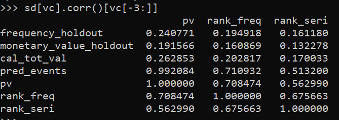
The correlation between pv and the holdout cumulative crime severity cal_tot_val, is not great at 0.26. But lets look at this relative to the more typical approach analysts will do, simply rank prior offenders based on either total number of events or the crime seriousness:

# Lets look at this method via just ranking prior
# seriousness or frequency
sd['rank_freq'] = sd['frequency_cal'].rank(method='first',ascending=True)
sd['rank_seri'] = (sd['monetary_value_cal']*sd['frequency_cal']).rank(method='first',ascending=True)
vc += ['rank_freq','rank_seri']
sd[vc].corr()[vc[-3:]]

So we can see that pv outperforms ranking based on total crimes (rank_freq), or ranking based on the cumulative serious score for offenders (rank_seri) in terms of the correlation for either the total number of future events or the cumulative crime harm.

If we look at capture rates, e.g. pretend we highlight the top 50 chronic offenders for intervention, we can see the criminal lifetime value pv estimate outperforms either simple ranking scheme by quite a bit:

# Look at capture rates by ranking
topn = 50
res_summ = []
for v in vc[-3:]:
    rank = sd[v].rank(method='first',ascending=False)
    locv = sd[rank <= topn].copy()
    tot_crimes = locv['frequency_holdout'].sum()
    tot_ser = locv['cal_tot_val'].sum()
    res_summ.append( [v,tot_crimes,tot_ser,topn] )

res_df = pd.DataFrame(res_summ,columns=['Var','TotCrimes','TotSer','TotN'])
res_df

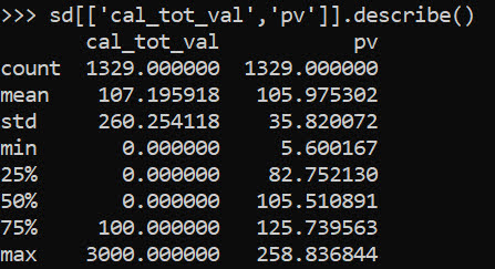
In terms of the seriousness projection, it is reasonably well calibrated over the entire sample, but has a very tiny variance – it basically just predicts the average crime serious score over the sample and assigns that as the prediction going forward:

# Cumulative stats over sample reasonable
# variance much too small
sd[['cal_tot_val','pv']].describe()

So what this means is that if say Chicago READI wanted to do estimates to reasonably justify the max dollar cost for their program (over a large number of individuals) that would be reasonable. And this is how most marketing people use this info, average benefits of retaining a customer.

For individual projections though, e.g. I think OffenderB will generate between [low,high] crime harm in the next year, this is not quite up to par. I am hoping though to pursue these models further, maybe either in a machine learning/regression framework to estimate the parameters directly, or to use mixture models in an equivalent way that marketers use “segmentation” to identify different types of customers. Knowing the different way people have formulated models though is very helpful to be able to build a machine learning framework, which you can incorporate covariates.

References

Staggered Treatment Effect DiD count models

So I have been dealing with various staggered treatments for difference-in-difference (DiD) designs for crime data analysis on how interventions reduce crime. I’ve written about in the past mine and Jerry’s WDD estimator (Wheeler & Ratcliffe, 2018), as well as David Wilson’s ORR estimator (Wilson, 2022).

There has been quite a bit of work in econometrics recently describing how the traditional way to apply this design to staggered treatments using two-way fixed effects can be misleading, see Baker et al. (2022) for human readable overview.

The main idea is that in the scenario where you have treatment heterogeneity (TH from here on) (either over time or over units), the two-way fixed effects estimator is a weird average that can misbehave. Here are just some notes of mine though on fitting the fully saturated model, and using post-hoc contrasts (in R) to look at that TH as well as to estimate more reasonable average treatment effects.

So first, we can trick R to use glm to get my WDD estimator (or of course Wilson’s ORR estimator) for the DiD effect with count data. Here is a simple example from my prior blog post:

# R code for DiD model of count data
count <- c(50,30,60,55)
post <- c(0,1,0,1)
treat <- c(1,1,0,0)

df <- data.frame(count,post,treat)

# Wilson ORR estimate
m1 <- glm(count ~ post + treat + post*treat,data=df,family="poisson")
summary(m1)

And here is the WDD estimate using glm passing in family=poisson(link="identity"):

m2 <- glm(count ~ post + treat + post*treat,data=df,
          family=poisson(link="identity"))
summary(m2)

And we can see this is the same as my WDD in the ptools package:

library(ptools) # via https://github.com/apwheele/ptools
wdd(c(60,55),c(50,30))

Using glm will be more convenient than me scrubbing up all the correct weights, as I’ve done in the past examples (such as temporal weights and different area sizes). It is probably the case you can use different offsets in regression to accomplish similar things, but for this post just focusing on extending the WDD to varying treatment timing.

Varying Treatment Effects

So the above scenario is a simple pre/post with only one treated unit. But imagine we have two treated units and three time periods. This is very common in real life data where you roll out some intervention to more and more areas over time.

So imagine we have a set of crime data, G1 is rolled out first, so the treatment is turned on for periods One & Two, G2 is rolled out later, and so the treatment is only turned on for period Two.

Period    Control     G1     G2
Base          50      70     40
One           60      70     50
Two           70      80     50

I have intentionally created this example so the average treatment effect per period per unit is 10 crimes. So no TH. Here is the R code to show off the typical default two-way fixed effects model, where we just have a dummy variable for unit+timeperiods that are treated.

# Examples with Staggered Treatments
df <- read.table(header=TRUE,text = "
 Period    Control     G1     G2
 Base          50      70     40
 One           60      70     50
 Two           70      80     50
")

# reshape wide to long
nvars <- c("Control","G1","G2")
dfl <- reshape(df,direction="long",
               idvar="Period",
               varying=list(nvars),
               timevar="Unit")

dfl$Unit <- as.factor(dfl$Unit)
names(dfl)[3] <- 'Crimes'

# How to set up design matrix appropriately?
dfl$PostTreat <- c(0,0,0,0,1,1,0,0,1)

m1 <- glm(Crimes ~ PostTreat + Unit + Period,
          family=poisson(link="identity"),
          data=dfl)

summary(m1) # TWFE, correct point estimate

The PostTreat variable is the one we are interested in, and we can see that we have the correct -10 estimate as we expected.

OK, so lets create some treatment heterogeneity, here now G1 has no effects, and only G2 treatment works.

dfl[dfl$Unit == 2,'Crimes'] <- c(70,80,90)

m2 <- glm(Crimes ~ PostTreat + Unit + Period,
          family=poisson(link="identity"),
          data=dfl)

summary(m2) # TWFE, estimate -5.29, what?

So you may naively think that this should be something like -5 (average effect of G1 + G2), or -3.33 (G1 gets a higher weight since it is turned on for the 2 periods, whereas G2 is only turned on for 1). But nope rope, we get -5.529.

We can estimate the effects of G1 and G2 seperately though in the regression equation:

# Lets seperate out the two units effects
dfl$pt1 <- 1*(dfl$Unit == 2)*dfl$PostTreat
dfl$pt2 <- 1*(dfl$Unit == 3)*dfl$PostTreat

m3 <- glm(Crimes ~ pt1 + pt2 + Unit + Period,
          family=poisson(link="identity"),
          data=dfl)

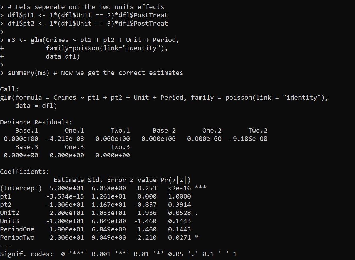
summary(m3) # Now we get the correct estimates

And now we can see that as expected, the effect for G2 is the pt2 coefficient, which is -10. And the effect for G1, the pt1 coefficient, is only floating point error different than 0.

To then get a cumulative crime reduction effect for all of the areas, we can use the multcomp library and the glht function and construct the correct contrast matrix. Here the G1 effect gets turned on for 2 periods, and the G2 effect is only turned on for 1 period.

library(multcomp)
cont <- matrix(c(0,2,1,0,0,0,0),1)
cumtreat <- glht(m3,cont) # correct cumulative
summary(cumtreat)

And if we want an ‘average treatment effect per unit and per period’, we just change the weights in the contrast matrix:

atreat <- glht(m3,cont/3) # correct average over 3 periods
summary(atreat)

And this gets us our -3.33 that is a more reasonable average treatment effect. Although you would almost surely just focus on that the G2 area intervention worked and the G1 area did not.

You can also fit this model alittle bit easier using R’s style formula instead of rolling your own dummy variables via the formula Crimes ~ PostTreat:Unit + Unit + Period:

But, glht does not like it when you have dropped levels in these interactions, so I don’t do this approach directly later on, but construct the model matrix and drop non-varying columns.

Next lets redo the data again, and now have time varying treatments. Now only period 2 is effective, but it is effective across both the G1 and G2 locations. Here is how I construct the model matrix, and what the resulting sets of dummy variables looks like:

# Time Varying Effects
# only period 2 has an effect

dfl[dfl$Unit == 2,'Crimes'] <- c(70,80,80)

# Some bookkeeping to make the correct model matrix
mm <- as.data.frame(model.matrix(~ -1 + PostTreat:Period + Unit + Period, dfl))
mm <- mm[,names(mm)[colSums(mm) > 0]] # dropping zero columns
names(mm) <- gsub(":","_",names(mm))  # replacing colon
mm$Crimes <- dfl$Crimes
print(mm)

Now we can go ahead and fit the model without the intercept.

# Now can fit the model
m6 <- glm(Crimes ~ . -1,
          family=poisson(link="identity"),
          data=mm)

summary(m6)

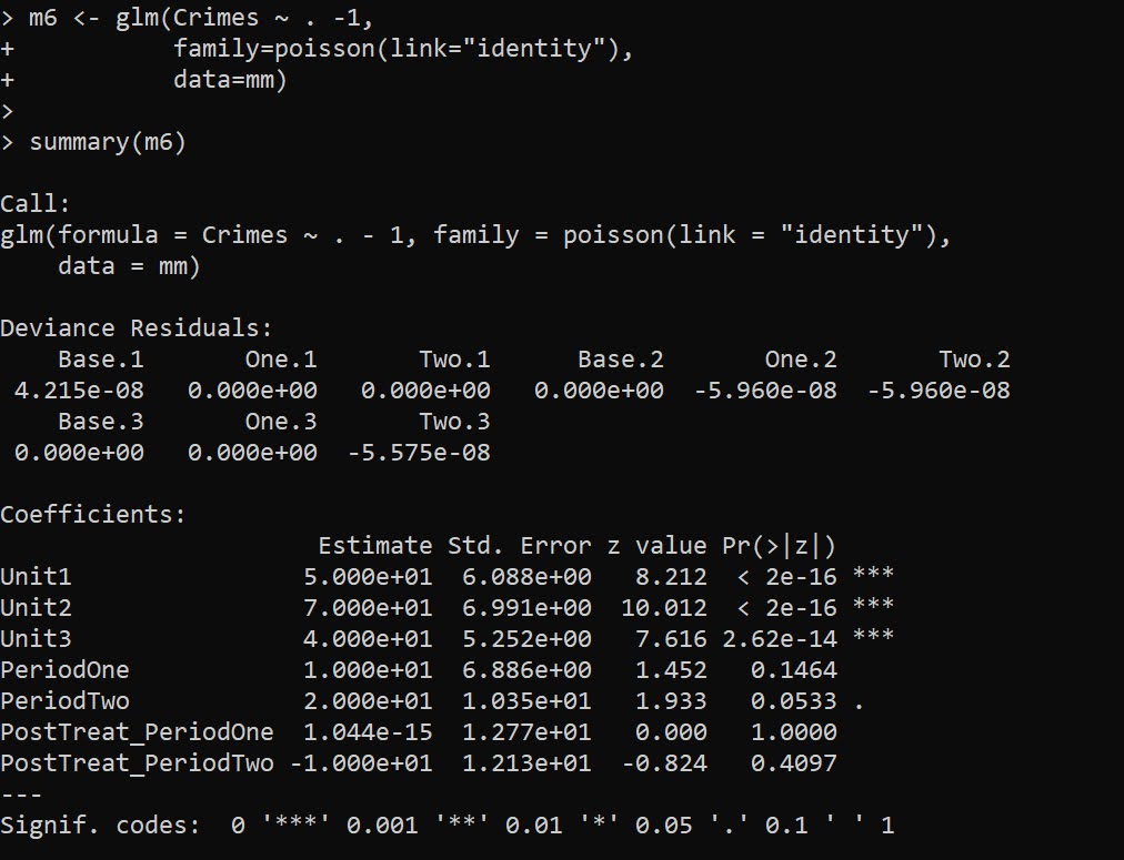
And you can see we estimate the correct effects here, PostTreat_PeriodOne has a zero estimate, and PostTreat_PeriodTwo has a -10 estimate. And now our cumulative crimes reduced estimate -20

cumtreat2 <- glht(m6,"1*PostTreat_PeriodOne + 2*PostTreat_PeriodTwo=0")
summary(cumtreat2)

And if we did the average, it would be -6.66.

Now for the finale – we can estimate the saturated model with time-and-unit varying treatment effects. Here is what the design matrix looks like, just a bunch of columns with a single 1 turned on:

# Now for the whole shebang, unit and period effects
mm2 <- as.data.frame(model.matrix(~ -1 + Unit:PostTreat:Period + Unit + Period, dfl))
mm2 <- mm2[,names(mm2)[colSums(mm2) > 0]] # dropping zero columns
names(mm2) <- gsub(":","_",names(mm2))  # replacing colon
mm2$Crimes <- dfl$Crimes
print(mm2)

And then we can fit the model the same way:

m7 <- glm(Crimes ~ . -1,
          family=poisson(link="identity"),
          data=mm2)

summary(m7) # Now we get the correct estimates

And you can see our -10 estimate for Unit2_PostTreat_PeriodTwo and Unit3_PostTreat_PeriodTwo as expected. You can probably figure out how to get the cumulative or the average treatment effects at this point:

tstr <- "Unit2_PostTreat_PeriodOne + Unit2_PostTreat_PeriodTwo + Unit3_PostTreat_PeriodTwo = 0"
cumtreat3 <- glht(m7,tstr)
summary(cumtreat3)

We can also use this same framework to get a unit and time varying estimate for Wilson’s ORR estimator, just using family=poisson with its default log link function:

m8 <- glm(Crimes ~ . -1,
          family=poisson,
          data=mm2)

summary(m8)

It probably does not make sense to do a cumulative treatment effect in this framework, but I think an average is OK:

avtreatorr <- glht(m8,
  "1/3*Unit2_PostTreat_PeriodOne + 1/3*Unit2_PostTreat_PeriodTwo + 1/3*Unit3_PostTreat_PeriodTwo = 0")
summary(avtreatorr)

So the average linear coefficient is -0.1386, and if we exponentiate that we have an IRR of 0.87, so on average when a treatment occurred in this data a 13% reduction. (But beware, I intentionally created this data so the parallel trends for the DiD analysis were linear, not logarithmic).

Note if you are wondering about robust estimators, Wilson suggests using quasipoisson, e.g. glm(Crimes ~ . -1,family="quasipoisson",data=mm2), which works just fine for this data. The quasipoisson or other robust estimators though return 0 standard errors for the saturated family=poisson(link="identity") or family=quasipoisson(link="identity").

E.g. doing

library(sandwich)
cumtreat_rob <- glht(m7,tstr,vcov=vcovHC,type="HC0")
summary(cumtreat_rob)

Or just looking at robust coefficients in general:

library(lmtest)
coeftest(m7,vcov=vcovHC,type="HC0")

Returns 0 standard errors. I am thinking with the saturated model and my WDD estimate, you get the issue with robust standard errors described in Mostly Harmless Econometrics (Angrist & Pischke, 2008), that they misbehave in small samples. So I am a bit hesitant to suggest them without more work to establish they behave the way they should in smaller samples.

References

  • Angrist, J.D., & Pischke, J.S. (2008). Mostly Harmless Econometrics. Princeton University Press.
  • Baker, A.C., Larcker, D.F., & Wang, C.C. (2022). How much should we trust staggered difference-in-differences estimates? Journal of Financial Economics, 144(2), 370-395.
  • Wheeler, A.P., & Ratcliffe, J.H. (2018). A simple weighted displacement difference test to evaluate place based crime interventions. Crime Science, 7(1), 1-9.
  • Wilson, D.B. (2022). The relative incident rate ratio effect size for count-based impact evaluations: When an odds ratio is not an odds ratio. Journal of Quantitative Criminology, 38(2), 323-341.

The limit on the cost efficiency of gun violence interventions

Imagine a scenario where someone came out with technology that would 100% reduce traffic fatalities at a particular curve in a road. But, installation and maintenance of the tech would cost $36 million dollars per 100 feet per year. It is unlikely anyone would invest in such technology – perhaps if you had a very short stretch of road that resulted in a fatality on average once a month it would be worth it. In that case, the tech would result in $36/12 = $3 million dollars to ‘save a life’.

There are unlikely any stretches of roads that have this high of fatality rate though (and this does not consider potential opportunity costs of less effective but cheaper other interventions). So if we had a location that has a fatality once a year, we are then paying $36 million dollars to save one life. We ultimately have upper limits on what society will pay to save a life.

Working on gun violence prevention is very similar. While gun violence has potentially very large costs to society, see Everytown’s estimates of $50k to a nonfatal shooting and $270k for a fatality, preventing that gun violence is another matter.

The translation to gun violence interventions from the traffic scenario is ‘we don’t have people at super high risk of gun violence’ and ‘the interventions are not going to be 100% effective’.

My motivation to write this post is the READI intervention in Chicago, which has a price tag of around $60k per participant per 20 months. What makes this program then ‘worth it’ is the probability of entrants being involved with gun violence multiplied by the efficacy of the program.

Based on other work I have done on predicting gun violence (Wheeler et al., 2019b), I guesstimate that any gun violence predictive instrument spread over a large number of individuals will have at best positive predictive probabilities of 10% over a year. 10% risk of being involved in gun violence is incredibly high, a typical person will have something more on the order of 0.01% to 0.001% risk of being involved with gun violence. So what this means is if you have a group of 100 high risk people, I would expect ~10 of them to be involved in a shooting (either as a victim or offender).

This lines up almost perfectly with READI, which in the control group had 10% shot over 20 months. So I think READI actual did a very good job of referring high risk individuals to the program. I don’t think they could do any better of a job in referring even higher risk people.

This though implies that even with 100% efficacy (i.e. anyone who is in READI goes to 0% risk of involvement in gun violence), you need to treat ~10 people to prevent ~1 shooting victimization. 100% efficacy is not realistic, so lets go with 50% efficacy (which would still be really good for a crime prevention program, and is probably way optimistic given the null results). Subsequently this implies you need to treat ~20 people to prevent ~1 shooting. This results in a price tag of $1.2 million to prevent 1 shooting victimization. If we only count the price of proximal gun violence (as per the Everytown estimates earlier), READI is already cost-inefficient from the get go – a 100% efficacy you would still need around 10 people (so $600k) to reduce a single shooting.

The Chicago Crime Lab uses estimates from Cohen & Piquero (2009) to say that READI has a return on investment of 3:1, so per $60k saves around $180. These however count reductions over the life-course, including person lost productivity, not just state/victim costs, which I think are likely to be quite optimistic for ROI that people care about. (Productivity estimates always seem suspect to me, models I have put into production in my career have generated over 8 digits of revenue, but if I did not do that work someone else would have. I am replaceable.)

I think it is likely one can identify other, more cost effective programs to reduce gun violence compared to READI. READI has several components, part of which is a caseworker, cognitive behavior therapy (CBT), and a jobs program. I do not know cost breakdowns for each, but it may be some parts drive up the price without much benefit over the others.

I am not as much on the CBT bandwagon as others (I think it looks quite a bit like the other pysch research that has come into question more recently), but I think caseworkers are a good idea. The police department I worked with on the VOID paper had caseworkers as part of their intervention, as did focused deterrence programs I have been involved with (Wheeler et al., 2019a). Wes Skogan even discussed how caseworkers were part of Chicago CEASEFIRE/outreach workers on Jerry Ratcliffe’s podcast. For those not familiar, case workers are just social workers assigned to these high risk individuals, and they often help their charges with things like getting an ID/Drivers License and applying to jobs. So just an intervention of caseworkers assigned to high risk people I think is called for.

You may think many of these high risk individuals are not amenable to treatment, but my experience is a non-trivial number of them are willing to sit down and try to straighten their lives out, and they need help to do that it. Those are people case workers are a good potential solution.

Although I am a proponent of hot spots policing as well, if we are just talking about shootings, I don’t think hot spots will have a good return on investment either (Drake et al., 2022). Only if you widen the net to other crimes do a think hot spots makes sense (Wheeler & Reuter, 2021). And maybe here I am being too harsh, if you reduce other criminal behavior READIs cost-benefit ratio likely looks better. But just considering gun violence, I think dropping $60k per person is never going to be worth it in realistic high gun violence risk populations.

References

Home buying and collective efficacy

With the recent large appreciation in home values, around 20% in the prior year, there have been an increase in private investors purchasing homes to rent out. Recent stories on this by Tyler Dukes and colleagues have collated open parcel data to identify the scope of these companies across all of North Carolina.

For bit of background, I tried to purchase a home in Plano, TX early 2018. Homes in our price range at that time were going in a single day and typically a few thousand over asking price.

Fast forward to early 2021, I am full remote data scientist instead of a professor, and kiddo is in online school. Even with the pay bump, housing competition was even worse in Plano at this point, so we knew we were likely going to have to move school districts to be able to purchase a home. So we decided to strike out, and ended up looking around Raleigh. Ended up quite quickly deciding to purchase a new build home in the suburb of Clayton (totally recommend our realtor, Ellen Pitts, her crew did quite a bit of work for us remotely).

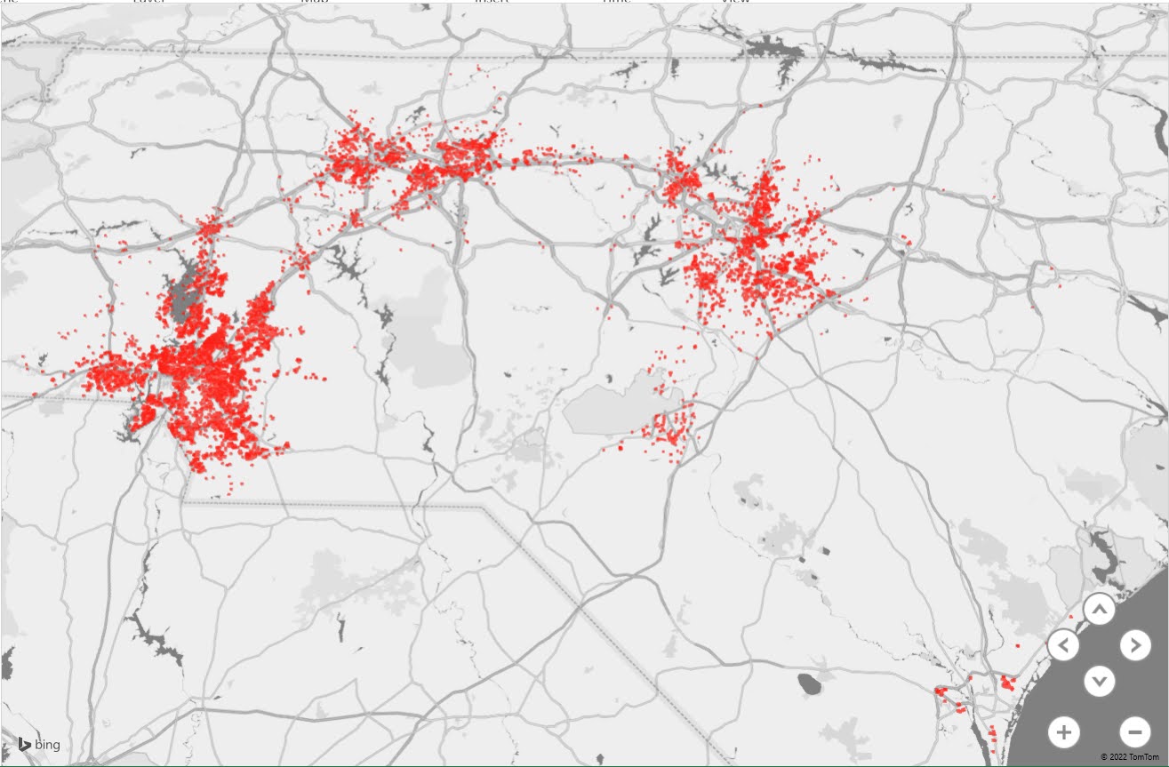
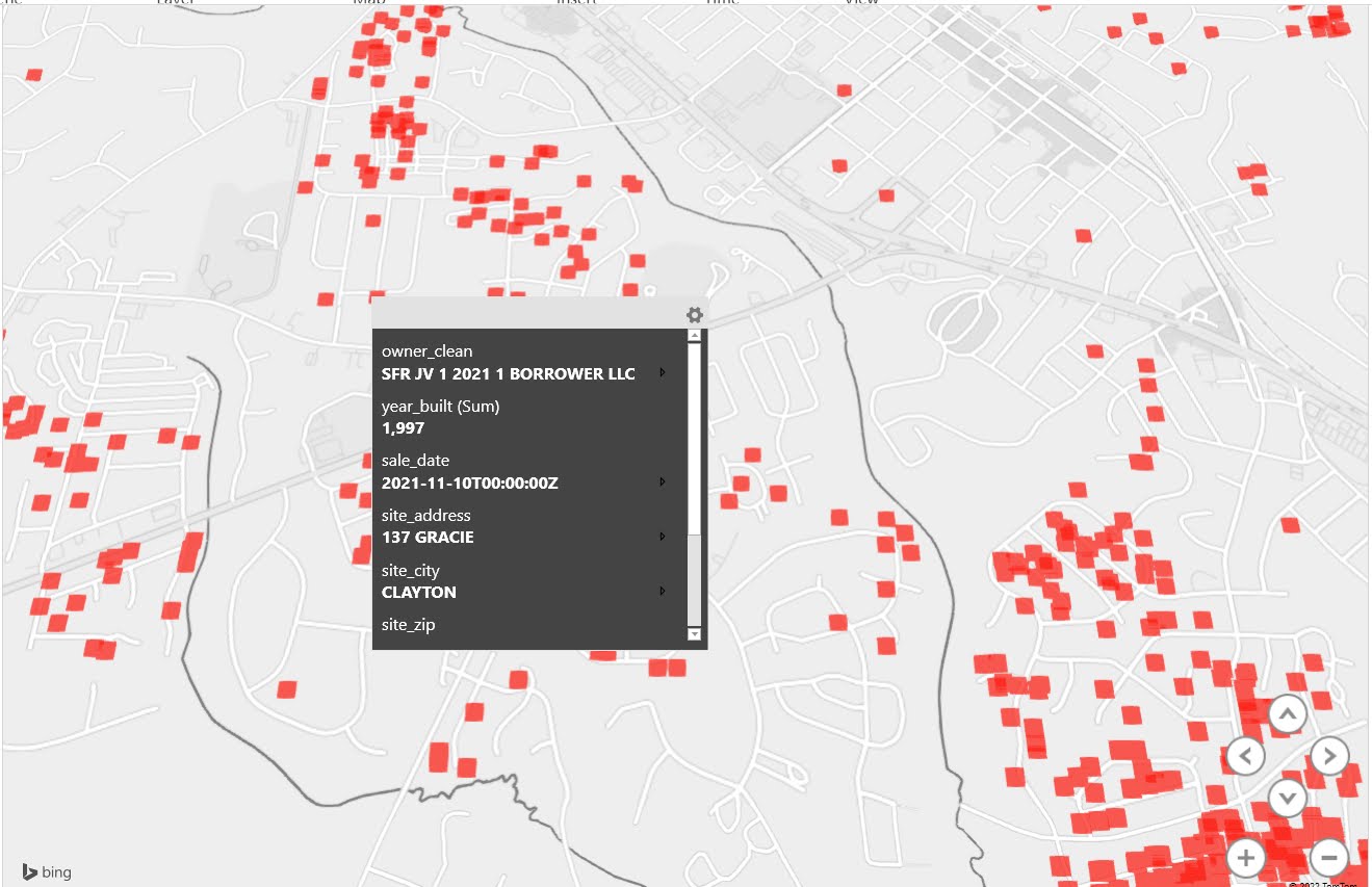
I was lucky to get in then it appears – many of the new developments in the area are being heavily scooped up by these equity firms (and rent would be ~$600 more for my home than the mortgage). So I downloaded the public data Dukes put together, and loaded it into Excel to make a quick map of the properties.

For a NC state view, we have big clusters in Charlotte, Greensboro and Raleigh:

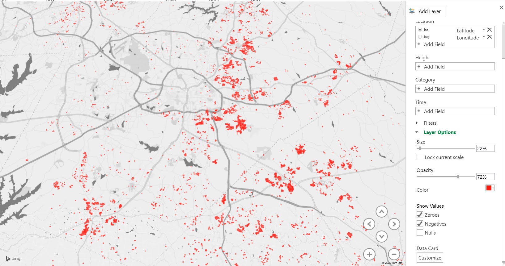
We can zoom in, and here is an overview of triangle area:

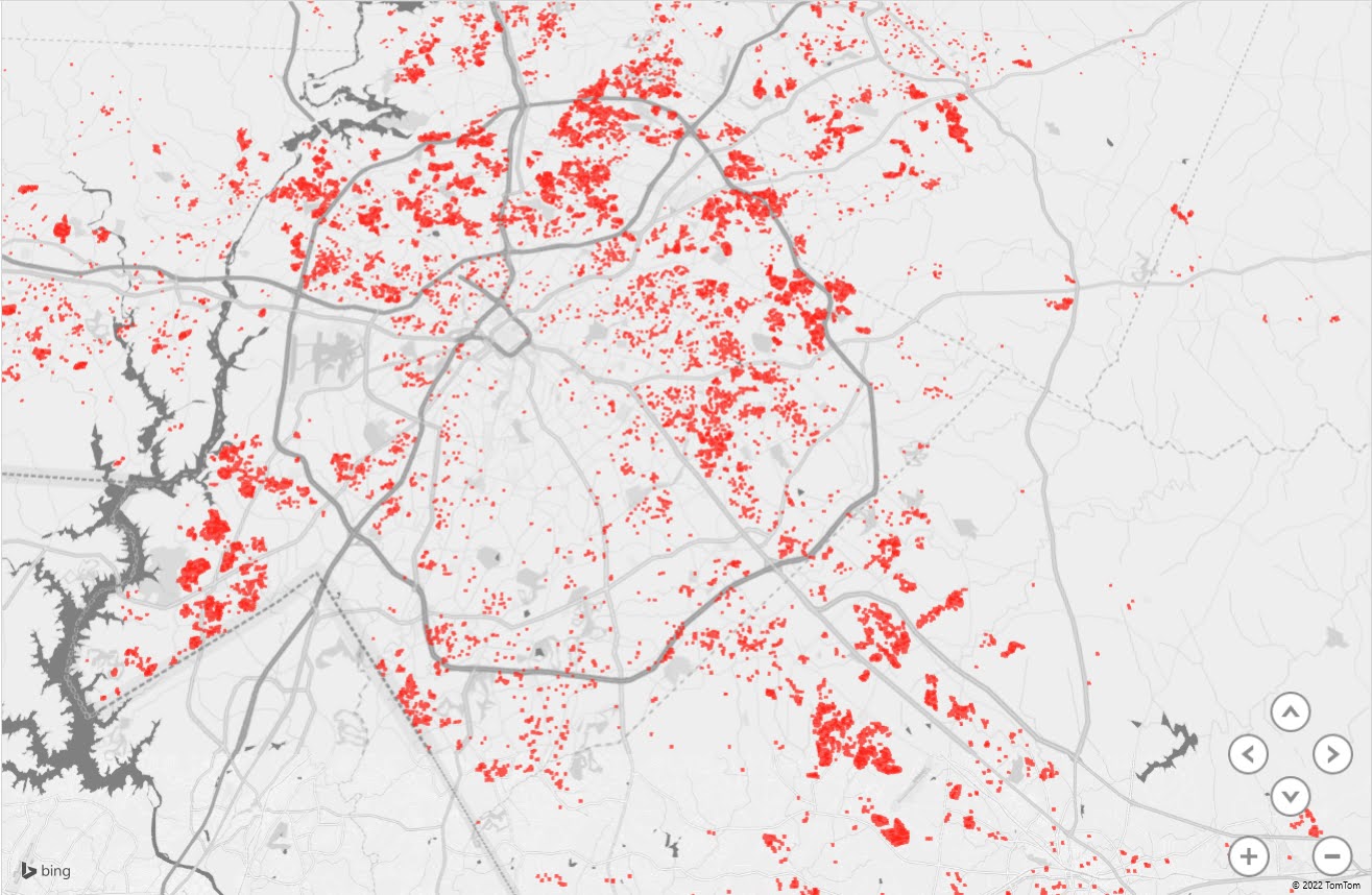
So you can see that inside the loop in Raleigh is pretty sparse, but many of the newer developments on the east side have many more of the private firm purchased houses. Charlotte is much more infilled with these private firms purchasing properties.

Zooming in even further to my town of Clayton, there is quite a bit of variance in the proportion of private vs residential purchases across various developments. My development is less than 50% of these purchases, several developments though appear almost 100% private purchased though. (This is not my home/neighborhood FYI.)


So what does this have to do with collective efficacy? Traditionally areas with higher home ownership have been associated with lower rates of crime. For not criminologists reading my blog, one of the most prominent criminological theories is that state actions only move the needle slightly on increasing/decreasing crime, people enforcing social norms is a bigger factor that explains high crime vs low crime areas. Places with people churning out more frequently – which occurs in areas with more renters – tend to have fewer people effectively keeping the peace. Because social scientists love to make up words, we call this concept collective efficacy.

Downloading and looking at this data, while I was mostly just interested in zooming into my neighborhood and seeing the infill of renters, sparked a criminological hypothesis: I expect neighborhoods with higher rates of private equity purchased housing in the long run to have higher rates of criminal behavior.

This hypothesis will be difficult to test in the wild. It is partially confounded with capital – those who buy their homes accumulate more wealth over time (again mortgage is quite a bit cheaper than rent, so even ignoring home value appreciation this is true). But the variance in the number of homes purchased by private equity firms in different areas makes me wonder if there is enough variation to do a reasonable research design to test my hypothesis, especially in the Charlotte area in say two or three years post a development being finished.

An update on the WaPo Officer Involved Shooting Stats

Marisa Iati interviewed me for a few clips in a recent update of the WaPo data on officer involved fatal police shootings. I’ve written in the past the data are very consistent with a Poisson process, and this continues to be true.

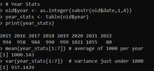
So first thing Marisa said was that shootings in 2021 are at 1055 (up from 1021 in 2020). Is this a significant increase? I said no off the cuff – I knew the average over the time period WaPo has been collecting data is around 1000 fatal shootings per year, so given a Poisson distribution mean=variance, we know the standard deviation of the series is close to sqrt(1000), which approximately equals 60. So anything 1000 plus/minus 60 (i.e. 940-1060) is within the typical range you would expect.

In every interview I do, I struggle to describe frequentist concepts to journalists (and this is no different). This is not a critique of Marisa, this paragraph is certainly not how I would write it down on paper, but likely was the jumble that came out of my mouth when I talked to her over the phone:

Despite setting a record, experts said the 2021 total was within expected bounds. Police have fatally shot roughly 1,000 people in each of the past seven years, ranging from 958 in 2016 to last year’s high. Mathematicians say this stability may be explained by Poisson’s random variable, a principle of probability theory that holds that the number of independent, uncommon events in a large population will remain fairly stagnant absent major societal changes.

So this sort of mixes up two concepts. One, the distribution of fatal officer shootings (a random variable) can be very well approximated via a Poisson process. Which I will show below still holds true with the newest data. Second, what does this say about potential hypotheses we have about things that we think might influence police behavior? I will come back to this at the end of the post,

R Analysis at the Daily Level

So my current ptools R package can do a simple analysis to show that this data is very consistent with a Poisson process. First, install the most recent version of the package via devtools, then you can read in the WaPo data directly via the Github URL:

library(devtools)
install_github("apwheele/ptools")
library(ptools)

url <- 'https://raw.githubusercontent.com/washingtonpost/data-police-shootings/master/fatal-police-shootings-data.csv'
oid <- read.csv(url,stringsAsFactors = F)

Looking at the yearly statistics (clipping off events recorded so far in 2022), you can see that they are hypothetically very close to a Poisson distribution with a mean/variance of 1000, although perhaps have a slow upward trend over the years.

# Year Stats
oid$year <- as.integer(substr(oid$date,1,4))
year_stats <- table(oid$year)
print(year_stats)
mean(year_stats[1:7]) # average of 1000 per year
var(year_stats[1:7])  # variance just under 1000

We can also look at the distribution at shorter time intervals, here per day. First I aggregat the data to the daily level (including 0 days), second I use my check_pois function to get the comparison distributions:

#Now aggregating to count per day
oid$date_val <- as.Date(oid$date)
date_range <- paste0(seq(as.Date('2015-01-01'),max(oid$date_val),by='days'))
day_counts <- as.data.frame(table(factor(oid$date,levels=date_range)))
head(day_counts)

pfit <- check_pois(day_counts$Freq, 0, 10, mean(day_counts$Freq))
print(pfit)

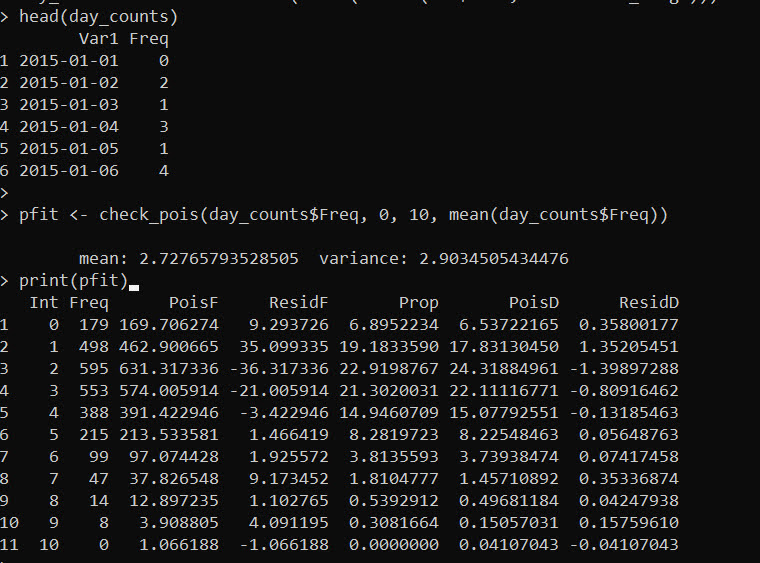
The way to read this, for a mean of 2.7 fatal OIS per day (and given this many days), we would expect 169.7 0 fatality days in the sample (PoisF), but we actually observed 179 0 fatality days, so a residual of 9.3 in the total count. The trailing rows show the same in percentage terms, so we expect 6.5% of the days in the sample to have 0 fatalities according to the Poisson distribution, and in the actual data we have 6.9%.

You can read the same for the rest of the rows, but it is mostly the same. It is only very slight deviations from the baseline Poisson expected Poisson distribution. This data is the closest I have ever seen to real life, social behavioral data to follow a Poisson process.

For comparison, lets compare to the NYC shootings data I have saved in the ptools package.

# Lets check against NYC Shootings
data(nyc_shoot)
date_range <- paste0(seq(as.Date('2006-01-01'),max(nyc_shoot$OCCUR_DATE),by='days'))
shoot_counts <- as.data.frame(table(factor(nyc_shoot$OCCUR_DATE,levels=date_range)))

sfit <- check_pois(shoot_counts$Freq,0,max(shoot_counts$Freq),mean(shoot_counts$Freq))
round(sfit,1)

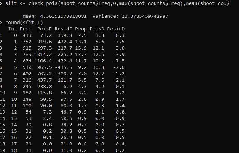
This is much more typical of crime data I have analyzed over my career (in that it deviates from a Poisson process by quite a bit). The mean is 4.4 shootings per day, but the variance is over 13. There are many more 0 days than expected (433 observed vs 73 expected). And there are many more high crime shooting days than expected (tail of the distribution even cut off). For example there are 27 days with 18 shootings, whereas a Poisson process would only expect 0.1 days in a sample of this size.

My experience though is that when the data is overdispersed, a negative binomial distribution will fit quite well. (Many people default to a zero-inflated, like Paul Allison I think that is a mistake unless you have a structural reason for the excess zeroes you want to model.)

So here is an example of fitting a negative binomial to the shooting data:

# Lets fit a negative binomial and check out
library(fitdistrplus)
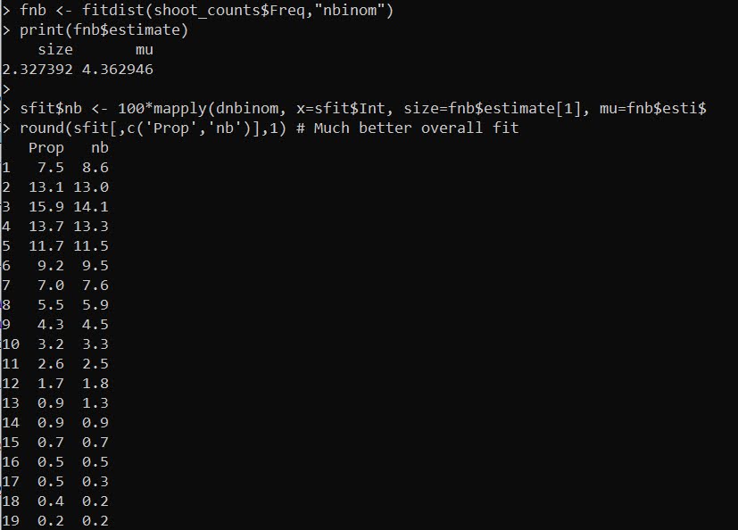
fnb <- fitdist(shoot_counts$Freq,"nbinom")
print(fnb$estimate)

sfit$nb <- 100*mapply(dnbinom, x=sfit$Int, size=fnb$estimate[1], mu=fnb$estimate[2])
round(sfit[,c('Prop','nb')],1) # Much better overall fit

And this compares the percentages. So you can see observed 7.5% 0 shooting days, and expected 8.6% according to this negative binomial distribution. Much closer than before. And the tails are fit much closer as well, for example, days with 18 shootings are expected 0.2% of the time, and are observed 0.4% of the time.

So What Inferences Can We Make?

In social sciences, we are rarely afforded the ability to falsify any particular hypothesis – or in more lay-terms we can’t really ever prove something to be false beyond a reasonable doubt. We can however show whether empirical data is consistent or inconsistent with any particular hypothesis. In terms of Fatal OIS, several ready hypotheses ones may be interested in are Does increased police scrutiny result in fewer OIS?, or Did the recent increase in violence increase OIS?.

While these two processes are certainly plausible, the data collected by WaPo are not consistent with either hypothesis. It is possible both mechanisms are operating at the same time, and so cancel each other out, to result in a very consistent 1000 Fatal OIS per year. A simpler explanation though is that the baseline rate has not changed over time (Occam’s razor).

Again though we are limited in our ability to falsify these particular hypotheses. For example, say there was a very small upward trend, on the order of something like +10 Fatal OIS per year. Given the underlying variance of Poisson variables, even with 7+ years of data it would be very difficult to identify that small of an upward trend. Andrew Gelman likens it to measuring the weight of a feather carried by a Kangaroo jumping on the scale.

So really we could only detect big changes that swing OIS by around 100 events per year I would say offhand. Anything smaller than that is likely very difficult to detect in this data. And so I think it is unlikely any of the recent widespread impacts on policing (BLM, Ferguson, Covid, increased violence rates, whatever) ultimately impacted fatal OIS in any substantive way on that order of magnitude (although they may have had tiny impacts at the margins).

Given that police departments are independent, this suggests the data on fatal OIS are likely independent as well (e.g. one fatal OIS does not cause more fatal OIS, nor the opposite one fatal OIS does not deter more fatal OIS). Because of the independence of police departments, I am not sure there is a real great way to have federal intervention to reduce the number of fatal OIS. I think individual police departments can increase oversight, and maybe state attorney general offices can be in a better place to use data driven approaches to oversee individual departments (like ProPublica did in New Jersey). I wouldn’t bet money though on large deviations from that fatal 1000 OIS anytime soon though.

The Big 2020 Homicide Increase in Context

Jeff Asher recently wrote about the likely 2020 increase in Homicides, stating this is an unprecedented increase. (To be clear, this is 2020 data! Homicide reporting data in the US is just a few months shy of a full year behind.)

In the past folks have found me obnoxious, as I often point to how homicide rates (even for fairly large cities), are volatile (Wheeler & Kovandzic, 2018). Here is an example of how I thought the media coverage of the 2015/16 homicide increase was overblown.

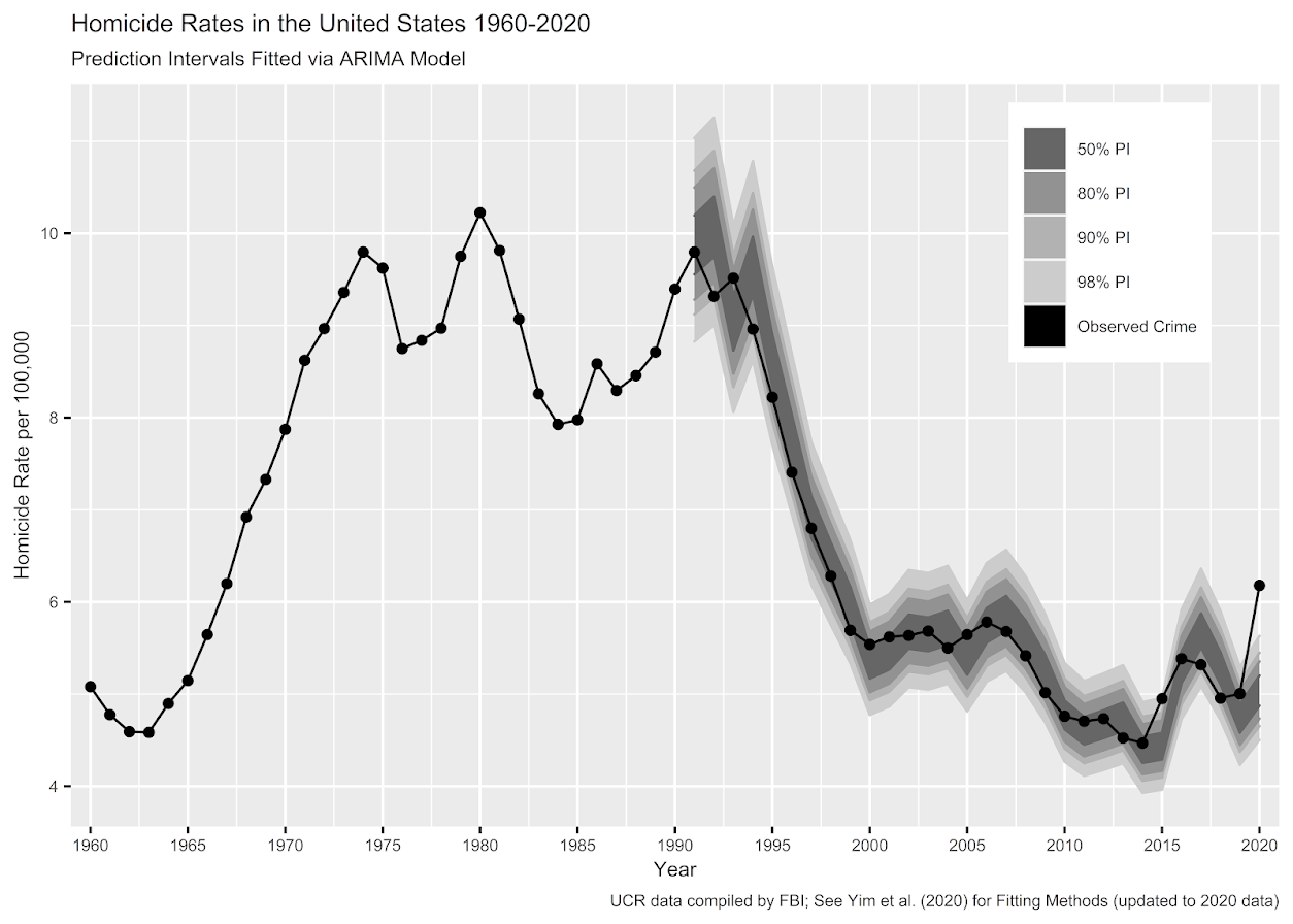
I actually later quantified this more formally with then students Haneul Yim and Jordan Riddell (Yim et al., 2020). We found the 2015 increase was akin to when folks on the news say a 1 in 100 year flood. So I was wrong in terms of it was a fairly substantive increase relative to typical year to year changes. Using the same methods, I updated the charts to 2020 data, and 2020 is obviously a much larger increase than the ARIMA model we fit based on historical data would expect:

Looking at historical data, people often argue “it isn’t as high as the early 90’s” – this is not the point though I really intended to make (it is kind of silly to make a normative argument about the right or acceptable number of homicides) – but I can see how I conflated those arguments. Looking at the past is also about understanding the historical volatility (what is the typical year to year change). Here this is clearly a much larger swing (up or down) than we would expect based on the series where we have decent US coverage (going back to 1960).


For thinking about crime spikes, I often come from a place in my crime analyst days where I commonly was posed with ‘crime is on the rise’ fear in the news, and needed to debunk it (so I could get back to doing analysis on actual crime problems, not imaginary ones). One example was a convenience store was robbed twice in the span of 3 days, and of course the local paper runs a story crime is on the rise. So I go and show the historical crime trends to the Chief and the Mayor that no, commercial robberies are flat. And even for that scenario there were other gas stations that had more robberies in toto when looking at the data in the past few years. So when the community police officer went to talk to that convenience store owner to simply lock up his cash in more regular increments, I told that officer to also go to other stores and give similar target hardening advice.

Another aspect of crime trends is not only whether a spike is abnormal (or whether we actually have an upward trend), but what causes it. I am going to punt on that – in short it is basically impossible in normal times to know what caused short term spikes absent identifying specific criminal groups (which is not so relevant for nationwide spikes, but even in large cities one active criminal group can cause observable spikes). We have quite a bit of crazy going on at the moment – Covid, BLM riots, depolicing – I don’t know what caused the increase and I doubt we will ever have a real firm answer. We cannot run an experiment to see why these increases occurred – it is mostly political punditry pinning it on one theory versus another.

For the minor bit it is worth – the time series methods I use here signal that the homicide series is ARIMA(1,1,0) – which means both an integrated random walk component and a auto-regressive component. Random walks will occur in macro level data in which the micro level data are a bunch of AR components. So this suggests a potential causal attribution to increased homicides is homicides itself (crime begets more crime). And this can cause run away effects of long upwards/downwards trends. I don’t know of a clear way though to validate that theory, nor any obvious utility in terms of saying what we should do to prevent increases in homicides or stop any current trends. Even if we have national trends, any intervention I would give a thumbs up to is likely to be local to a particular municipality. (Thomas Abt’s Bleeding Out is about the best overview of potential interventions that I mostly agree with.)

References

  • Wheeler, A. P., & Kovandzic, T. V. (2018). Monitoring volatile homicide trends across US cities. Homicide Studies, 22(2), 119-144.
  • Yim, H. N., Riddell, J. R., & Wheeler, A. P. (2020). Is the recent increase in national homicide abnormal? Testing the application of fan charts in monitoring national homicide trends over time. Journal of Criminal Justice, 66, 101656.

Notes for the 2019/2020 updated homicide data. 2019 data is available from the FBI page, 2020 homicide data I have taken from estimates at USA Facts and total USA pop is taken from Google search results.

R code and data to replicate the chart can be downloaded here.

Musings on Project Organization, Books and Courses

Is there a type of procrastination via which people write lists of things? I have that condition.

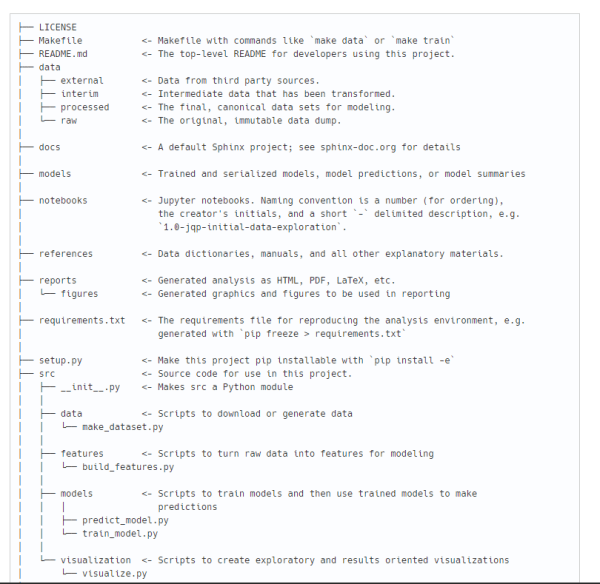
I have been recently thinking about project organization. At work we have been using the Cookie Cutter Data Science project set up – and I really hate it. I have been thinking about this more recently, as I have taken over several other data scientists models at work. The Cookie Cutter Template is waaaay too complicated, and mixes logic of building python packages (e.g. setup.py, a LICENSE folder) with data science in production code (who makes their functions pip installable for a production pipeline?). Here is the Cookie Cutter directory structure (even slightly cut off):

Cookie cutter has way too many folders (data folder in source, and data folder itself), multiple nested folders (what is the difference between external data, interim, and raw data?, what is the difference between features and data in the src folder?) I can see cases for individual parts of these needed sometimes (e.g. an external data file defining lookups for ICD codes), but why start with 100 extra folders that you don’t need. I find this very difficult taking over other peoples projects in that I don’t know where there are things and where there are not (most of these folders are empty).

So I’ve reorganized some of my projects at work, and they now look like this:

├── README.md           <- High level overview of project + any special notes
├── requirements.txt    <- Default python libraries we often use (eg sklearn, sqlalchemy)
├                         + special instructions for conda environments in our VMs
├── .gitignore          <- ignore `models/*.pkl`, `*.csv`, etc.
├── /models             <- place to store trained and serialized models
├── /notebooks          <- I don't even use notebooks very often, more like a scratch/EDA folder
├── /reports            <- Powerpoint reports to business (using HMS template)
├── /src                <- Place to store functions

And then depending on the project, we either use secret environment variables, or have a YAML file that has database connection strings etc. (And that YAML is specified in .gitignore.)

And then over time in the root folder it will typically have shell scripts call whatever production pipeline or API we are building. All the function files in source is fine, although it can grow to more modules if you really want it to.

And this got me thinking about how to teach this program management stuff to new data scientists we are hiring, and if I was still a professor how I would structure a course to teach this type of stuff in a social science program.

Courses

So in my procrastination I made a generic syllabi for what this software developement course would look like, Software & Project Development For Social Scientists. It would have a class/week on using the command prompt, then a week on github, then a few weeks building a python library, then ditto for an R package. And along the way sprinkle in literate programming (notebooks and markdown and Latex), unit testing, and docker.

And here we could discuss how projects are organized. And social science students get exposed to way more stuff that is relevant in a typical data science role. I have over the years also dreamt up other data science related courses as well.

Stats Programming for CJ. This goes through the basics of data manipulation using statistical programming. I would likely have tutorials for R, python, SPSS, and Stata for this. My experience with students is that even if they have had multiple stats classes in grad school, if you ask them “take this incident dataset with dates, and prepare a weekly level file with counts of crimes per week” they don’t know how to do even that simple task (an aggregation). So students need an entry level data manipulation course.

Optimization for Criminal Justice (or alt title Operations Research and Machine Learning for CJ). This one is not as developed as some of my other courses, but I think I could make it work for a semester. I think learning linear programming is a really great skill not taught at all in any CJ program I am aware of. I have some small notes on machine learning in my Research Design class for PhD students, but that could be expanded out (week for decision trees/forests, week for boosting, week for neural networks, etc.).

And last, I have made syllabi for the one credit entry level course for undergrad students, and the equivalent course for the new PhD students, College Prep. These classes I had I don’t think did a very good job. My intro one at Bloomsburg for undergrad had a textbook lol! The only thing I remember about my PhD one was fear mongering over publications (which at that point I had no idea what was going on), and spending the last class with Julie Horney and David McDowell at whatever the place next to the Washington Tavern in Albany was called (?Gingerbread?).

These are of course just in my head at the moment. I have posted my course materials over the years that I have delivered.

I have pitched to a few programs to hire me as a semi teaching professor (and still keep my private sector gig). This set up is not that uncommon in comp sci departments, but no CJ ones I think are interested. Even though I like musing about courses, adjunct pay is way too low to justify this investment, and should be paid to both develop the material as well as deliver the class.

Books

I have similarly made outlines for books over the years as well. One is Data Science for Crime Analysis with Python. I think there is an opening in the crime analysis market to advance to more professional coding, and so a python book would be good. But the market is overall tiny, my high end guesstimates are only around 800, so hard to justify the effort. (It would be mainly just a collection of my blog posts, but all in a nicer format for everyone to walk through/replicate.)

Another is a reader book, Handbook of Advanced Crime Analysis. That may not be needed though, as Cory Haberman and Liz Groff did a recent book that has quite a bit of overlap (can’t find it at the moment, maybe it is not out yet). Many current advanced techniques are scattered and sometimes difficult to replicate, I figured a reader that also includes code walkthroughs would help quite a few PhD students.

And again if I was still in the publishing game I would like to turn my Poisson course notes into a little Sage green book.

If I was still a professor, this would go hand in hand with developing courses. I know Uni’s do sometimes have grants to develop open source teaching materials, and these would probably best fit those molds. These aren’t going to generate revenue directly from sales.

So complaints and snippets on blog posts are all you are going to get for now from me.

Spatial consistency of shootings and NIJ recid working papers

I have two recent working papers out:

The NIJ forecasting paper is the required submission by NIJ. Gio and I will likely try to turn this into a real paper in the near future. I’d note George Mohler and Michael Porter did the same thing as us, clip the probabilities to under 0.5 to win the fairness competition.

NIJ was interested in “what variables are the most important” – I will need to slate a longer blog post about this in the future, but this generally is not the right way to frame predictive challenges. You do not need real in depth understanding of the underlying system, and many times different effects can be swapped out for one another (e.g. Dawes, 1979).

The paper on shootings in Buffalo is consistent with my blog posts on shootings in NYC (precincts, grid cells). Even though shootings have gone up by quite a bit in Buffalo overall, the spatial distribution is very consistent over time. Appears similar to a recent paper by Jeff Brantingham and company as well.

It is a good use case for the differences in SPPT results when adjusting for multiple comparisons, we get a S index of 0.88 without adjustments, (see below distribution of p-values). These are consistent with random data though, so when doing a false discovery rate correction we have 0 areas below 0.05.

If you look at the maps there are some fuzzy evidence of shifts, but it is quite weak overall. Also one thing I mention here is that even though we have hot spots of shootings, even the hottest grid cells only have 1 shooting a month. Not clear to me if that is sufficient density (if only considering shootings) to really justify a hot spots approach.

References

  • Brantingham, P. J., Carter, J., MacDonald, J., Melde, C., & Mohler, G. (2021). Is the recent surge in violence in American cities due to contagion?. Journal of Criminal Justice, 76, 101848.
  • Circo, G., & Wheeler, A. (2021). National Institute of Justice Recidivism Forecasting Challenge Team “MCHawks” Performance Analysis. CrimRxiv. https://doi.org/10.21428/cb6ab371.9aa2c75a
  • Dawes, R. M. (1979). The robust beauty of improper linear models in decision making. American Psychologist, 34(7), 571.
  • Drake, G., Wheeler, A., Kim, D.-Y., Phillips, S. W., & Mendolera, K. (2021). The Impact of COVID-19 on the Spatial Distribution of Shooting Violence in Buffalo, NY. CrimRxiv. https://doi.org/10.21428/cb6ab371.e187aede
  • Mohler, G., & Porter, M. D. (2021). A note on the multiplicative fairness score in the NIJ recidivism forecasting challenge. Crime Science, 10(1), 1-5.

Potential IT student projects with police? (AMA)

Abigail White writes in:

I’m still settling in at my agency and getting an analysis program rolling. Before I came here, I volunteered with a nonprofit and I had partnered 2 years running with a local university to provide real-world opportunities for their 4th-year undergrad IT students to do a final project. Basically, I was the project owner and they were supposed to build an application, modify software for my needs, or do some project along those lines to get on-the-ground experience. The school just reached out again and asked if I wanted to do a project with them again this year with whatever organization I’m currently working with.

I really want to tell them yes because it’s a tremendous opportunity for these students to know about how IT can interface with the field of law enforcement (and to get some IT minds working on law enforcement problems). Plus my agency actually may want to hire in-house IT at some point so it could be a good way for them to screen some people and make a job offer at the end of the school year.

Do you have any ideas for projects that would be good to build bridges between the IT industry and law enforcement? I need to come up with something good before I pitch it to command. The best I can think of so far is a phone-based app where officers could record the lat and long of their exact location and add info about the environment around them – ultimately so we could start getting good data for risk terrain modeling (i.e., at this location, there’s an abandoned house, at another location, there’s an unoccupied house where the lawn hasn’t been mown, etc.) I know that’s not much to go on, but I would love to hear any thoughts you have!

And here is what I said off-the-cuff in response:

It is hard for me to gauge feasibility. In terms of app maybe a nice public facing dashboard (maps/charts), with public info. Can pitch as something for community group meetings for example. That is a good marriage between IT (worrying about the server) and crime analysis (queries to feed the dashboard) I think.

Phone app to me sounds too hard. Even if you build it very difficult to get data security down and the PD to actually use it. Public dashboard is for everyone and no security worries. (Building a phone app seems pretty far outside what an IT person would typically do within a PD.)

RTM in terms of building a predictive model is feasible, but making a nice way for the PD to consume it is more difficult (so is more traditional crime analysis type stuff). But could maybe make sense just internally.

I have seen someone try to do the video narratives with officers (similar to your app idea, just using gopro). It is neat, but not sure it results in very actionable intelligence to be honest.

This is just me rambling though. Typically for projects I start with something the PD will find useful based on my own observations. So would look for regular things done low-tech now by the PD that can maybe be automated or improved upon with some coding work.

Sharing here with the hopes others will have more ideas. It is similar in scope to say a really good undergrad or a masters level thesis type project I would say as well.

ptools R package

It has been on my bucket list for a bit, but I wanted to take the time to learn how to construct an R package (same as for a python package). So I crafted a package with only a few functions in it so far, ptools, short for Poisson tools.

These are a handful of functions I have blogged about over the years, including functions for various WDD tests and the variants I have blogged about (weighted harm scores, different time periods, and different area sizes).

Small sample counts in bins (which can be used for Benford’s test), or my original application was checking if a chronic offender had a propensity to commit crimes on certain days of the week.

The Poisson e-test, and a function to check whether a distribution is Poisson distributed and two more Poisson related functions as well.

I think I will add quite a few more functions in the soup before I bother submitting to CRAN. (Installing via devtools via github is quite easy, so I do not feel too bad about that.) If you have functions you think I should add just let me know. (Or just make a pull request and add them yourself!) I also need to work on unit tests, and getting github actions set up. I will probably crunch on this for a bit, and then migrate personal projects back to creating some python libraries for my other work.

I do not use R-studio, but the open book R packages has been immensely helpful. On my windows box I had to bother to add R to my system path, so I can start my R session at the appropriate directory, but besides that very minor hassle it has been quite easy to follow.


I probably have not put in my 10k total hours as a guesstimate to mastery in computer programming. I think maybe closer to 5000, and that is spread out (maybe quite evenly at this point) between python, R, SPSS (and just a little Stata). And I still learn new stuff all the time. Being in an environment where I need to work with more people has really hammered down getting environments right, and making it shareable with other teammates. And part and parcel with that is documenting code in a much more thorough manner than most of the code snippets I leave littered on this blog.

So it probably is worth me posting less, but spending more time making nicer packages to share with everyone.

I do not know really how folks do R programming for making packages. I know a little at this point about creating separate conda environments for python to provide some isolation – is there something equivalent to conda environments for R? Do the R CMD checks make this level of isolation unnecessary? Should I just be working on an isolated docker image for all development work? I do not know. I do not have to worry about that at the moment though.


Part of this self learning journey is because I am trying to start a journal aimed at criminologists where you can submit software packages. Similar to the Journal of Open Source Software or the Journal of Statistical Software, etc. For submission to there I want people to have documentation for functions, and really that necessitates having a nice package (whether in R or python or whatever). So I can’t tell people you need to make a package if I don’t do that myself!

The software papers are not a thing yet (I would call it a soft launch at this point), but I have been bugging folks about submitting papers to get a dry run of the process. If you have something you would like to submit, feel free to get in touch and we can get you set up.